Image Processing Reference
In-Depth Information
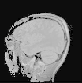
Original Image
Corrected Image
500
400
300
200
Optimization
of Histogram Metric
100
200
400
600
800
1000
Histogram
Inhomogeneity Field
Metric Computation
Tissue-Class Model
FIGURE 5.5
Schematic illustration of histogram-based inhomogeneity correction meth-
ods. In an optimization process (red arrows), the shape of the inhomogeneity field is
adapted such that the chosen metric computed from the histogram of the corrected image
is minimal. For the case of the PABIC method, an additional prior tissue-class model is
needed for the computation of the histogram metric (dashed arrow).
PABIC assumes that images are composed of regions with piecewise con-
stant intensities of mean values
σ
k
. Each voxel of
the idealized signal corrupted by noise must take values close to one of these
class means. These assumptions are violated by effects like partial voluming
and the natural inhomogeneity of biological tissue. To account for these vio-
lations, PABIC incorporates a robust M-estimator [49] function
f
k
(16) into the
histogram metric
e
tot
(17) (see Figure 5.6). Thanks to the robust estimator,
µ
k
and standard deviation
Energy function
Energy function
m
0
1
e
1
e
0.8
f
m
1
m
2
m
0
m
1
m
2
0.8
0.8
0.6
0.6
0.6
0.4
0.4
0.4
0.2
0.2
0.2
x
500
x
7
x
4
4
−
6
−
−
2
2
6
100
200
300
400
1
2
3
(b)
4
5
6
(a)
(c)
FIGURE 5.6
(a) Robust estimator function (Equation 5.16) for µ = 0 and σ = 2. (b) Three-
class energy function
e
(Equation 5.17) for σ
1
= σ
2
= σ
3
= 0.03, 0.1, 0.3 and 1.0, from
top to bottom respectively. (c) Example energy function
e
from a head MRI correction.


Search WWH ::

Custom Search