Retrospective Evaluation and Correction of Intensity Inhomogeneity - Advance Image Processing in Magnetic Resonance Imaging - page 149

classify

update inhomogeneity

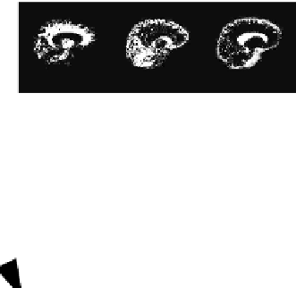
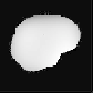
FIGURE 5.3 In the EM approach of Wells et al., inhomogeneity field estimation is

repeatedly interleaved with tissue classification, yielding improved results at each iteration.

that the estimates typically stabilize in five to ten iterations, after which the
algorithm is stopped. Upon convergence, an inhomogeneity field corrected image
can be obtained by subtracting the estimated inhomogeneity field from the log-
transformed intensities

and transforming the result back into the original MR
intensity domain using the exponential transformation.
Although Wells et al. showed excellent results on MR images of the brain,
a number of shortcomings were quickly identified, spawning a considerable
amount of papers aiming at improving upon the original method. One line of
research has concentrated on improving the segmentation results produced by the
algorithm, in particular, by employing so-called Markov random field (MRF)
models to minimize the effects of noise in the resulting segmentations [23-29].
While a detailed treatise of these methods is outside the scope of this text, suffice
it here to say that they encourage neighboring voxels to be classified to the same
tissue type, at the expense of making the E step computationally intractable,
necessitating approximative solutions. Another area of improvement upon the
original Wells algorithm involves the manual selection of a number of represen-
tative points for each of the tissues considered in order to estimate appropriate
values of the Gaussian distribution parameters

y

and Although it is straight-
forward to estimate these parameters for large well-defined regions such as white
and gray matter in brain MRI, other regions consist of several different types of
tissue, some of which are easily overlooked during training. Guillemaud and

µ σ 2 .

k