Hardware Reference
In-Depth Information
Tabl e 2. 1
Bridging defects
Guaranteed range .K/
Total number of bridges
Rb 0:5
258 (64.5%)
Rb 1
379 (94.8%)
Rb 5
394 (98.5%)
Rb 10
397 (99.3%)
Rb 20
400 (100%)
Guaranteed range
.
K
/
Total number of bridges
Rb 0:5
14 (3.5%)
Rb 1
12 (3.0%)
Rb 5
4 (1.0%)
Rb 10
2 (0.5%)
Rb 20
0(0%)
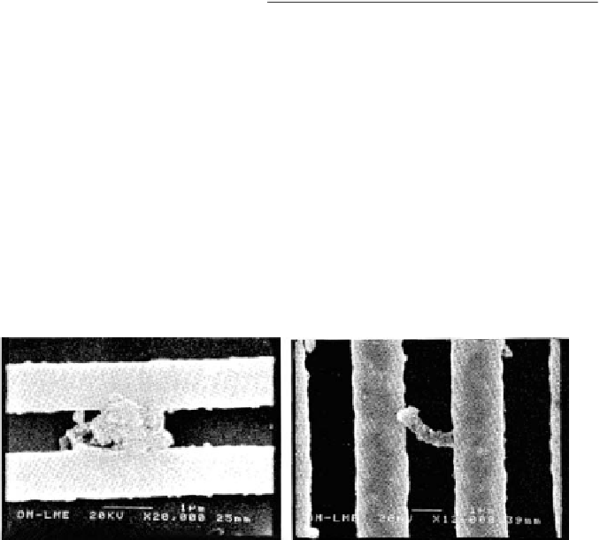
Fig. 2.7
(
a
) Low resistive and (
b
) high resistive bridging defect
(
Rodrıguez-Monta nes et al.
1996
)
side, 3.5% of the bridges have a resistance above 500 . The maximum resistance
value was found to be around 20 k. Two pictures of a low resistive and a high
2.3
Detectability of Bridging Defects
As the quality demands increase, the effectiveness of test generation without any
defect consideration becomes questionable. High quality test generation requires a
better knowledge of defect behaviour. As a matter of fact, the analysis of defect be-
haviour is a quite difficult task. One of the main difficulties comes from the presence
in the defect of random value parameters such as the bridging resistance preventing
any prediction of the defect behaviour. The mechanisms of defect appearance are
obviously not controlled, resulting in electrical situations with unknown parame-
ters. The question is how to predict the voltage created by a bridge when the value
of the bridge resistance is not known a priori. The classical assumptions such as