Geology Reference
In-Depth Information
Hillslope Evolution
Rules
Regolith
Production
Rule
B
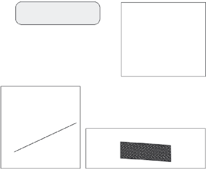
Fig. 11.5
Schematic illustration of
the components of a hillslope
evolution model that might be used
to assess scarp evolution.
A. Topographic,
z
(
x
), and bedrock,
z
b
(
x
), profiles, with in general a
non-uniform regolith thickness,
R
(
x
).
B. Regolith production rule, in which
the rate,
w
, is here taken to be
dependent only on the local regolith
thickness. C. Hillslope regolith specific
discharge rule, one in which the
discharge is linearly proportional to
the local slope of the landscape.
D. Mass balance on a regolith element
depends on the rate of rock-to-regolith
conversion,
w
, which adds mass to the
base of the element, and on the
downslope sediment flux both in to,
Q
x
, and out of,
Q
x
+d
x
, the element.
Surface and Bedrock
Topographic Profiles
A
w
o
z(x)
R*
z
b
(x)
Regolith Thickness, R
w
w
C
Hillslope
Flux Rule
R
Q = -k (dz/dx)
D
Mass Balance on a Regolith Element
dx
Q
x
Q
x+dx
Slope |dz/dx|
w dx
where
t
c
is the shear stress necessary to entrain
the sediment. Because the shear stress (
t
b
=
r
gHS
)
requires a knowledge of the flow depth,
H
, most
model strategies rewrite this rule in terms of the
water discharge,
Q
, which is a quantity that is
more directly tied to the climatic forcing of the
landscape. This assumption results in a yet sim-
pler statement:
most often a lack of datable material. In these
circumstances, researchers have turned to theo-
retical models of how a scarp is expected evolve
in the face of the surface processes active on it.
The idea is simple: because, in most cases, scarp
shape evolves monotonically from sharp-edged
toward smoother forms (Nature abhors sharp
corners), a knowledge of the initial shape of the
scarp and documentation of the detailed shape
of the scarp, through surveying in the field, may
be used to estimate the age of the feature.
Q
s
=
cQ
(11.5)
Examples
Theory
Given the set of rules stated above, a wide array
of models can be generated that differ in their
initial and boundary conditions, and in the
pattern of uplift and subsidence imposed by
tectonic processes. We start with simple fault-
scarp models in the next section and then move
to larger features.
Starting with the extensive work of Culling in
the 1960s (Culling, 1960, 1963, 1965), most mod-
els are based on the diffusion equation. A useful
introduction can also be found in Carson and
Kirkby (1972). In direct analogy with the well-
understood thermal problem (Carslaw and
Jaeger, 1986), the relevant equations derive from
two statements: (i) mass is conserved, and (ii)
the flux of mass is proportional to the local top-
ographic slope (Fig. 11.5). The first statement
may be written, for the one-dimensional case, as
Scarp degradation modeling
In many instances, none of the absolute dating
methods discussed in Chapter 3 can be applied
to a particular landform, be it a fault scarp, a
lake shoreline, or a marine terrace. The reason is
∂
∂
z
1
Q
(11.6)
=−
x
∂
r
∂
t
x
b