Geology Reference
In-Depth Information
At any point along a river profile, the change in
height with time,
δ
z
/
δ
t
, is the difference between
rock uplift,
U
, and erosion (Eqn 8.4), such that
Equilibrium Profiles: Concavity Index
A
δ
z
/
δ
t
=
U
−
E
=
U
−
KA
m
S
n
(8.5)
In this context,
K
amalgamates many different
variables that control erosional efficiency,
including rock erodibility, sediment load, climate,
erosion process, hydraulic geometry, and the
return period for effective discharges. Even
though many of these variables are usually
poorly known, the effects of changes in some of
them are commonly predictable: weaker rocks,
higher rainfall, and shorter return periods
should all lead to more rapid erosion for any
given area or channel slope.
For a steady-state profile in which channel
elevation at a point does not change,
δ
z
/
δ
t
equals zero, and Eqn 8.5 can be rearranged in
terms of the equilibrium slope,
S
e
, as follows:
S
e
=
(
U
/
K
)
1/
n
A
−
m
/
n
Normalized Distance from Divide
Equilibrium Profiles: Steepness Index
B
(8.6)
Distance from Divide (m)
If
U
and
K
are constant, then the ratio
m
/
n
defines the rate of change of channel gradient
as a function of drainage area. In other words,
the long profile of the river is a function of
m
/
n
,
which is defined as the
concavity
and is typically
designated as
q
. A channel with no concavity
represents a linear gradient, whereas a channel
with high concavity will have steep headwaters
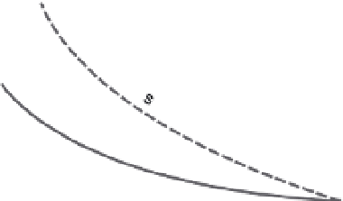
and gentle downstream slopes (Fig. 8.4).
For the purposes of analyzing river networks
using DEMs, Eqn 8.6 is commonly recast as
Fig. 8.4
Channel concavity and steepness.
A. Channel concavity, expressed as the ratio of
m
/
n
in
the formulation for channel slope (Eqn 8.6). Inset shows
how channel slope changes as a function of drainage
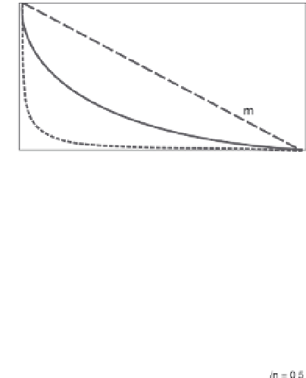
area for different concavities. B. Despite identical
concavity values (
m
/
n
=
0.5; see inset), these profiles
have different gradients as reflected by their steepness
index,
k
s
, in Eqn 8.7. The steepness index is defined by
the
y
intercept in log slope-log area space (inset).
Modified after Duvall
et al.
(2004).
diverse DEMs. When data for channel slope
versus upstream catchment area are systemati-
cally plotted in log-log space, several key channel
characteristics typically emerge (Fig. 8.5). First,
at small catchment areas, slope may be largely
independent of area. This region is considered
to be either hillslopes or channels where
processes such as debris flows, rather than river
incision, dominate erosion (Stock and Dietrich,
2006). Second, at a certain critical area that is
equivalent to about 1 km
2
(or 10
6
m
2
) in many
studies (
A
c
in Fig. 8.5), the fluvial channel head is
recognized by the start of a progressive decrease
in channel slope. Third, in many analyses, this
decrease can be fit by a line with a slope that is
equivalent to the channel concavity,
q
or
m
/
n
.
S
=
k
s
A
−
q
(8.7)
where
k
s
is the
steepness index
and equals
(
U
/
K
)
1/
n
(Whipple
et al
., 1999; Wobus
et al
.,
2006c). The steepness index in relation to
U
/
K
makes intuitive sense: for any given catchment,
we would expect channel steepness to increase
for higher uplift rates (Fig. 8.3B) or to decrease
for weaker rocks or more rainfall. Our intuition,
however, can sometimes fool us. In looking at
the profiles in Fig. 8.4B, many people would
deduce that profile B has higher concavity,
whereas in fact both profiles have identical
concavities, but different steepness indices.
The utility of channel indices like concavity or
steepness becomes obvious when applied to