Graphics Programs Reference
In-Depth Information
load population.dat
year = population(:,1);
P = population(:,2);
plot(year,P,':o')
box;grid
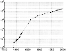
The European population prior to 1850 was very low and we are unable
to see the fine detail. Detail is revealed when we use a logarithmic
y
-
scale:
semilogy(year,P,':o')
box;grid
The following functions implement logarithmic axes:
loglog
Both axes logarithmic
semilogx
logarithmic
x
-axis
semilogy
logarithmic
y
-axis
14 Curve Fitting—Matrix Division
We continue with the example of Australian population data given in
the previous section. Let us see how well a polynomial fits this data. We
assume the data can be modelled by a parabola:
p
=
c
0
+
c
1
x
+
c
2
x
2
where
x
is the year,
c
0
,
c
1
, and
c
2
are coeQcients to be found, and
p
is
the population. We write down this equation substituting our measured
data:
p
1
=
c
0
+
c
1
x
1
+
c
2
x
1
p
2
=
c
0
+
c
1
x
2
+
c
2
x
2
.
.
.
p
N
=
c
0
+
c
1
x
N
+
c
2
x
2
N