Graphics Programs Reference
In-Depth Information
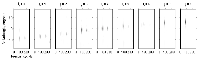
You can see that over the 8 time steps, the arrival direction of the sound
has changed from
45 degrees to 30 degrees, and the two sources always
come from the same direction, strengthening our notion that the two are
in fact harmonics of the same source. Let us look at the time-frequency
and time-angle distributions of this data. The above output of the
whos
command shows that the row index of
data
corresponds to the different
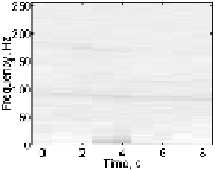
angles, so if we calculate the mean over the rows we will be left with a
time-frequency distribution:
−
>> time_freq = mean(data);
>> size(time_freq)
ans =
1
1039
We are left with a 1
9 matrix of averages over the 128 arrival
angles. To plot the results we have to squeeze this to a two-dimensional
103
×
103
×
×
9 matrix:
time_freq = squeeze(mean(data));
imagesc(t,f,time_freq)
axis xy
xlabel('Time, s')
ylabel('Frequency, Hz')
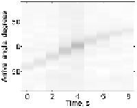
The frequency varies slightly with time. By averaging the rows of the
data matrix we can get a similar plot of the variation of arrival angle
with time:
time_angle = squeeze(mean(data,2));
imagesc(t,th,time_angle)
axis xy
xlabel('Time, s')
ylabel('Arrival angle, degrees')
29.5 Multidimensional Cell Arrays
Multidimensional cell arrays are just like ordinary multidimensional
arrays, except that the cells can contain not only numbers, but vectors,