Graphics Programs Reference
In-Depth Information
>> whos
Name
Size
Bytes Class
data
128x103x9
949248 double array
f
1x103824 double array
t
1x9
72 double array
th
1x128
1024 double array
The data consists of spectra measured at 103 frequencies, 128 arrival
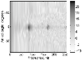
angles, and 9 time steps. Let us plot the fifth time sample:
colormap(flipud(gray))
imagesc(f,th,data(:,:,5))
axis xy
colorbar
xlabel('Frequency, Hz')
ylabel('Arrival angle, degrees')
Darker colours correspond to higher intensities. You can see two strong
sources at an angle of zero degrees and at frequencies of 85 and 170 Hz.
The fact that 170 = 2
85 might lead us to suspect that the 170 Hz
source is just the first harmonic of the 85 Hz source. Let us look at all of
the time samples together. This time we'll cut off the lower intensities
by setting the minimum colour to correspond to an intensity of 5 (this
is the call to
caxis
in the following code). We also turn off the
y
-axis
tick labels for all but the first plot, and we make the tick marks point
outwards:
10
×
for i = 1:9
subplot(3,9,i), imagesc(f,th,data(:,:,i)), axis xy
set(gca,'tickdir','out')
ifi==1
ylabel('Arrival angle, degrees')
xlabel('Frequency, Hz')
end
if i>1, set(gca,'yticklabel',[]), end
caxis([5 Inf]), title(['i_t = ' num2str(t(i))])
end
10
See Handle Graphics Sections 23 and 31 (pages 63 and 107).