Civil Engineering Reference
In-Depth Information
or
S
i
1
/m
Δ
S
re
=
λ
i
Δ
.
(5.55)
3 is the root mean cube (RMC) probability density func-
tion describing the effective constant amplitude stress range distribution,
Equation 5.55 with
m
=
S
re
, that
causes the same amount of fatigue damage as the design variable amplitude stress
range distribution (e.g., the mid-span bending moment for Cooper's E80 load shown
in
Figure 5.34)
.
No FS is applied since the Palmgren-Miner linear damage accumu-
lation rule is considered relatively accurate for service level highway and railway
live loads (Fisher, 1984).An example of determining the effective constant amplitude
stress range from a variable amplitude load is shown in Example 5.19.
Δ
Example 5.19
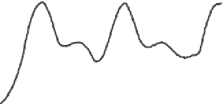
Determine the effective constant amplitude stress range,
S
re
, for the vari-
able amplitude stress spectrum shown in
Figure E5.17
(the variable amplitude
Cooper's E80 design loading on a 25 ft long span shown in
Figure 5.34
).
The peak stresses corresponding to the variable amplitude loads are
shown in
Table E5.5
and
Figure E5.18.
Rainflow cycle counting is performed
as indicated in Figure E5.18 and
Table E5.6.
Four complete stress range cycles (eight half-cycles) are present (
N
Δ
=
4).
Calculation of the effective constant amplitude stress range,
Δ
S
re
, is shown
in
Table E5.7.
S
re
=
g
i
(
Δ
S)
3
=
(
509.7
)
1
/
3
Δ
=
8.0 ksi.
Equation 5.55 indicates that the railway fatigue design load must be expressed
in terms of the number of cycles and magnitude of load. The fatigue design load
recommended by AREMA (2008) is based on analyses of continuous unit freight
Cooper's E80 mid-span flexural stress trace
(25 ft span)
20
18
16
14
12
10
8
6
4
2
0
05
10
15
20
25
30
Time
FIGURE E5.17