Geography Reference
In-Depth Information
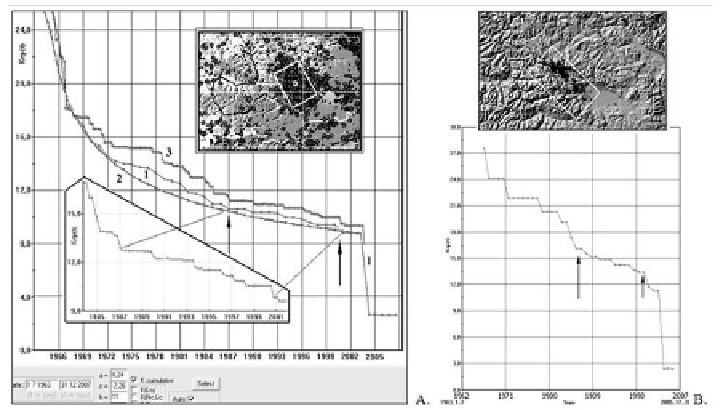
Figure 7. A - Time series of rupture density
K
avg
[35] for the Chuya earthquake area,
M
s
≥ 2
: 1) real curve with
∆T
= 1 year, 2) theoretical curve of uniform fracture growth
(
∆T
= 1 year), 3) real curve with
∆T
= 1 month shifted upward. Arrows show
coincidence of curves 1 and 2. Box frames a fragment corresponding to the period
between 1987 and 2000 when the real curve flattened out with
ΔT
= 3 months. B - real
curve of
K
avg
for the Chuya earthquake area,
M
s
≥
2.5
. The curves have become
smoother since 1986 and fall abruptly since 2000.
The module for calculating the parameter of environment damage or
seismic rupture density
K
avg
(t)
(Figure 7) was designed one of the latest among
the graphic methods. The time series of this parameter provide an idea of
seismic stability reflected in physical changes of the environment. The
stability is understood as uniform increment of rupture length and number of
earthquakes.
The cartographical methods imply contour line mapping, animation
cartography (visualizing earthquakes as gradually fading flares spaced at time
intervals proportional to real time) and constructing vertical cross sections and
patterns of elevation and seismicity (Figure 8).
The built-in mapping subsystem unit can produce cartograms showing
distribution of such seismicity parameters as total seismic energy, which is
useful to highlight zones of quiescence preceding large earthquakes;
distribution of the
b
parameter (slope of recurrence curve); maps of energy
stability (
K
avg
) and its rms error σ; contour lines of seismic activity (
A
10
,
A
15
,
where
A
is a long-term average number of earthquakes of certain energy:
K
=
10, 15) (as, for example, the
K
avg
map in Figure 9).