Geography Reference
In-Depth Information
•
unlike the
classical
case (Figure 6 B, c) of calculating the elliptic
metrics, it is suggested to create an ellipse of equal probability (Figure
6 B, a).
In the third method, called
interactive
, the space-time window values (
dS
and
dT)
are set up by the user. The results of the
elliptic
method are considered
below in more detail (Figure 6).
In the
elliptical
method, which includes the described steps, the following
parameters are set up: threshold signal/noise ratio
R
s/n
, minimum main shock
magnitude, minimum aftershock magnitude, minimum size of the rectangular
metric, etc. The
classical
way of finding the ellipse parameters [29] may be
with or without weighting (Figures 6 B,
b
and
c
), which depends on the
number of events that fall into the cell. Weighting makes sense if aftershock
swarms are strongly scattered.
Experience has shown that, in some cases, our
modified
method of
identifying aftershocks may be advantageous, in which ithe spatial pattern of
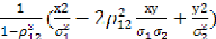
aftershocks is constrained by an equal probability ellipse:
= const =
2
,
(х,у) =
where
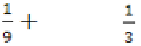
2
2 · ( 1
)
3
is approximation of the quintile
3.29 ·
distribution with two degrees of freedom at Р = 0.9995; = DX, = DY -
are the variances of
х
and
у
, and is the correlation coefficient between
х
and
у
. Thus estimated ellipse parameters for identifying aftershocks of the
09.16.2003 earthquake in the northern Baikal Rift Zone (BRZ) exceeded those
obtained by the
classical
way in both number of selected events (263 and 246
respectively) and aftershock sequence length (3.9 and 1.6 times, respectively, -
Figure 6 B, e). Another advantage of our
modified
method is that the results
are almost independent of the
R
s/n
threshold.
The
classical
and
modified
aftershock removal algorithms were compared
in terms of efficiency by estimating the statistics of the resulting sets (Figure 6
B, f). The
classical
removal of aftershocks has shown significant deviation of
the observed distribution from the theoretical Poissonian distribution [30] both
before (Figure 6 B, f - 1), and after the procedure (Figure 6 B, f - 2), while the
modified
algorithm shows no deviation (Figure 6 B, f - 3).
The exponential Poisson distribution is given by: