Geography Reference
In-Depth Information
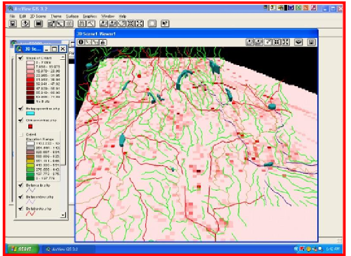
Figure 5. Detail of Slope Gradient analysis using Arcview 3.2 (L.C. Hazell).
The darker pixels indicated the steeper gradients and generally these are gradients
which modern roads or tracks follow.
The analysis could have been undertaken empirically by simply reading
the contours on the map or trace likely routes that showed minimal grades and
then marking these on photocopied survey maps. But this would have
necessitated either assessing contour spacing visually or measuring and
calculating the grade along a multitude of potential pathways. The study area
exhibits complex landforms, reflecting their volcanic origins. Using the slope
gradient tool in ArcView ensured consistent analyses. This is particularly
valuable when working with large areas and small-scale maps. Slope is
defined by pixel size. Adobe Photoshop pixel counts and grid value tools
determined the ground area that each pixel represented on our maps. Therefore
a linear distance of: ±40 m on 1:250000 scale maps; ±16 m at 1:50000 and ±4
m for 1:16000 per pixel applied in our maps.
To manually sample slope grades at these scales would require analysis of
each change of contour value across a potential pathway. The total fall from
the source to the floodplain is some 400m in vertical height with contour