Environmental Engineering Reference
In-Depth Information
segments of the boundary with the new correspondent ones
from aerial image if it exists. If there are several edge line
segments in a buffer zone, their slope and length will be
analyzed to determine the new ones. If there is not one in the
buffer zone, the old one is retained.
5
To refine the new boundary by least-squares template match-
ing with orthogonal constraints.
to 1 if the roof surfaces
P
i
and
P
j
are adjacent to each other.
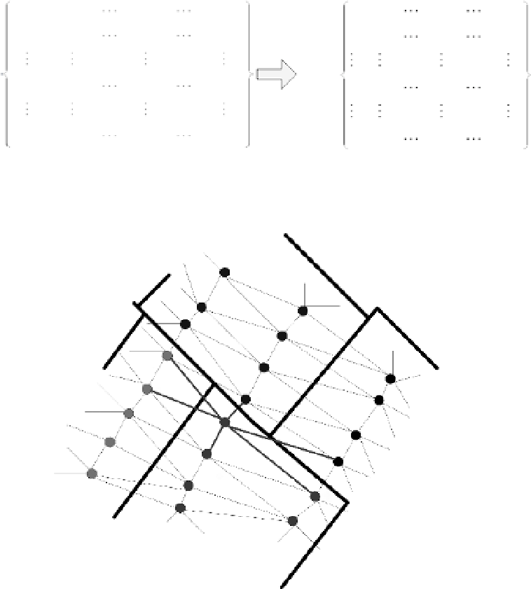
Otherwise, it will be labelled to 0. In Fig. 6.8(b), the diagonal
elements of the adjacent relationship matrix are set to 0 because
it is symmetric. It can be reconstructed with the help of the TIN
data structure. For example, given a point
V
m
within the surface
P
i
,findoutallofitsadjacentpoints
.As
showninFig.6.9,points
v
0
and
v
1
are located within surfaces
P
k
and
P
j
, respectively, and points
v
2
and
v
3
are both within surface
P
m
, so the value of
R
i
,
j
,
R
i
,
k
and
R
i
,
m
in the matrix equals to 1,
where,
i
,
j
and
k
are the indices of the roof surfaces.
With the aid of adjacent matrix, the small adjacent roof sur-
faces are merged according to their normal vectors. In general,
the threshold of merging surfaces is set to 5
◦
.Inotherwords,
if the angle of the normal vectors of the two adjacent surfaces
is smaller than this threshold, these two surfaces are merged.
For reconstruction of a 3D building model, normally building
corners are reconstructed first because they are the primitives of
a computer-aided drafting (CAD) model. Thus, the new rela-
tionship between roofs and vertical walls is remodeled by adding
the vertical walls into the adjacent matrix of the roof surfaces.
For each single line segment of a building boundary, we
first find all roof surfaces, then expand along its perpendicular
direction to form a buffer zone. According to the building points
within the buffer zone belonging to which one of the roof
surfaces, the adjacency of the vertical walls and roof surfaces can
be detected. Figure 6.10(a) shows an example of a building with
{
v
0
,
v
1
,
v
2
,
v
3
,
v
4
,
v
5
}
6.2.3.5
Computation of buildingmodels
The adjacency relationship of roof surfaces will be set up to
the reconstruction of 3D building model after detecting the
roof surfaces by an adjacent matrix graph. Under the adjacent
matrix relationship graph, the small adjacent roof surfaces were
merged if its normal vectors meet the predefined threshold. Then
line segments of boundary are treated as vertical walls to add
into adjacent matrix graph, from which the ridge points will be
decided by the intersection of adjacent surfaces and the building
corners will be calculated. Finally, the 3D building models can be
reconstructed.
Assume a set of roof surfaces
P
i
(
i
=
0, 1
...n
−
1) are
detected, the adjacency matrix can be represented as shown
in Fig. 6.8(a), where,
n
is the number of the roof surfaces,
R
i
,
j
(
i
=
0, 1,
...n
−
1;
j
=
0, 1,
...n
−
1) is the adjacency
relationship between
P
i
and
P
j
, whose elements will be labelled
0
R
0,1
R
0,
j
R
0,
n
−
1
R
0,0
R
0,1
R
0,
j
R
1,
j
R
0,
n
−
1
R
1,1
R
1,
n
−
1
R
1,
j
R
1,
n
−
1
R
1,0
00
R
n,n
=
R
n,n
=
R
i
,0
R
i
,1
R
i, j
R
i,n
−
1
00
0
R
i,n
−
1
R
n
-1,1
R
n
-1,0
R
n
-1,
j
R
n
-1,
n
-1
00
0
0
(a)
(b)
FIGURE 6.8
Adjacent matrix graph of roof surfaces.
v
2
P
m
P
j
V
3
V
1
P
k
v
4
v
0
P
i
v
5
FIGURE 6.9
An example of searching neighborhood.


Search WWH ::

Custom Search