A pluralistic approach to defining and measuring urban sprawl - Urban Remote Sensing: Monitoring, Synthesis and Modeling in the Urban Environment - page 165

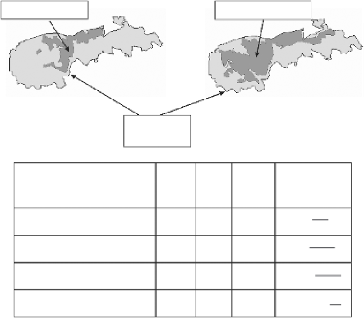
Built area - 1989 Built area - 2004

Municipal
Boundary

Sprawl Indexes 1989 2004 %

change

Equation

P i

D gi =

Gross density (residents per sq) 6,487 5,286 − 19%

UA i

L i
p A i

SH i =

Shape index (SH) 3.0 3.3 12%

2

√

Aout i
UA i

− 50% LFI gi =

Leap frog index (LFI) 2% 1%

a ij
n ij

n

Mean Patch Size (Ha) (MPS) 36.4 73.0 101%

MPS ij = ∑

= 1

Where:
P i = number of residents in urban settlement i
A i = centralbuilt-up area of urban settlement i

UA i = urban built-up area of settlement i

RA i = Residential area of settlement i (land-use no. 1)

L i = Perimeter of central built-up area of settlement i

Aout i = leapfrog areas in settlement i

a ij = area of land-use j in urban settlement i ( j = 1...n)

n ij = number of polygons of land-use j in urban settlement i
(j

1...n)

=

FIGURE 12.1 A temporal comparison of urban spatial growth for the Israeli city of Carmiel, 1989 and 2004. The built space
area estimated using maps and verified with aerial photographs and ground survey. Four sprawl measures are provided for
the two dates to compare temporal trends.

spatial data be available for two or more points in time, so
that temporal changes in spatial variables can be measured (see
Fig. 12.1). With regard to the second consideration, the user must
reconcile the tradeoff between low resolution needed to capture
large areas and for comparative research between regions, and
high resolution needed to capture fine-grained processes that
would be lost when resolution is too low (Irwin and Bockstael,
2008). An example of this tradeoff is the utility of Landsat data:
Landsat provides excellent data for large areas with high fre-
quency of data capture, but it lacks the resolution to capture
very low density development (Orenstein et al ., 2010). Low den-
sity development is of utmost importance when considering the
extent of sprawl (Irwin and Bockstael, 2008).
Third, by ranking individual sprawl measures, we do not
imply that a single measure will suffice in capturing this multi-
faceted phenomenon. On the contrary, since sprawl has so many
dimensions, simultaneous application of multiple indicators is
not only recommended, but required (Torrens and Alberti, 2000;
Galster et al ., 2001; Ewing, Pendall and Chen, 2002; Hasse and
Lathrop, 2003a; Sutton, 2003; Cutsinger and Galster, 2006). It is
apparent that quantitative indicators for measuring sprawl yield
ambiguous and often contrary results. Urban areas could be con-
sidered sprawled using some measures, yet compact using others

(Hasse, 2004; Frenkel and Ashkenazi, 2008b; Torrens, 2008). This
fact is exemplified through the use of four urban areas in Israel
(Fig. 12.2). In the figure, the ''Type A'' urban area ranks compact
using four sample sprawl measures. The ''type D'' urban area,
on the other hand, ranks sprawled using these measures. Types
B and C both rank sprawled on two of the four measures, but
they are different measures in both cases. This point is further
emphasized in the previous figure (Fig. 12.1), where over time at
one location, population density and shape index both suggest
more sprawl, while leapfrog index and mean patch size suggests
less sprawl. Clearly the use of one or even two measures misses
the complexity of sprawl characterization.
In response to this challenge, researchers are measuring mul-
tiple sprawl characteristics simultaneously (Ewing, Pendall and
Chen, 2002; Hasse and Lathrop, 2003a; Hasse, 2004; Irwin and
Bockstael, 2008; Frenkel and Ashkenazi, 2008b; Torrens, 2008),
or integrating multiple measures into a single index after nar-
rowing down the range of variables using reduction techniques
(Ewing, Pendall and Chen, 2002; Frenkel and Ashkenazi, 2008b).
Cutsinger and Galster (2006) argue that since metropolitan areas
may be considered sprawled according to some indicators while
simultaneously considered not sprawled in other dimensions, a