Object Tracking over Multiple Uncalibrated Cameras Using Visual, Spatial and Temporal Similarities - Advanced Concepts for Intelligent Vision Systems - page 169

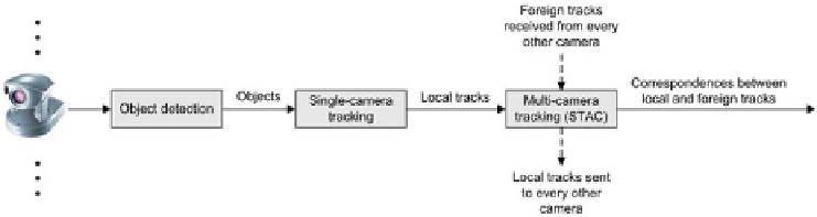
Fig. 1. A block diagram of the STAC algorithm running on a camera in a parallel
multi-camera tracking framework

Constructing the local kernel and local track snapshot. We use a 2D
Gaussian distribution to represent the kernel of a tracked object. This Gaussian
form will be used for finding spatial and temporal similarities between linked
pairs of kernels in section 2.2. The centre of the Gaussian distribution is located
at the centre of the object, and the standard deviation in the x and y directions
are equal to half the object's height and width, respectively. Each local cam-
era keeps a history of locally observed kernels of any tracked object previously
observed in this camera.
For each frame in which the tracked object is visible, the local track snapshot of
the tracked object is constructed. The local track snapshot contains: the kernel of
the tracked object in the current frame of the local camera; the object's signature
in the current frame of the local camera; the local track ID, as determined by
the single-camera tracker; and the current frame, f . This local track snapshot
is sent to every camera in the network. Consequently, the local camera receives
track snapshots from each foreign camera each frame, which we will call foreign
track snapshots . The local camera stores the foreign track snapshots over time
for use in linking kernels in the local camera to kernels in foreign cameras.

Reusing kernels. Creating a new kernel for each tracked object in every frame
causes the number of kernels to grow rapidly, resulting in large demands on
computing and memory resources. To overcome this, and to allow for historical
tracking statistics to be collected, an existing kernel is reused if a tracked object
has a similar position and size to a previously observed object. A similarity
score, s , is calculated between the potential new kernel and each existing kernel,
as detailed below.
The Euclidean distance, d , between the centres ( x 1 , y 1 )and( x 2 , y 2 )ofthe
potential new kernel and existing kernels, as well as the angle θ between the two
centres, are determined by,
d = ( x 2 − θ =tan − 1 y 2 −

y 1

x 1 ) 2 +( y 2 − y 1 ) 2 ,

. (1)

x 2 − x 1

Then, the standard deviations σ 1 and σ 2 of the potential new kernel and existing
kernel in the direction θ are calculated, which are given by (these equations are
derived from the polar equation of an ellipse),