A New System for Event Detection from Video Surveillance Sequences - Advanced Concepts for Intelligent Vision Systems - page 113

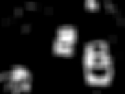
optical flow velocity and applicate of a gaussian filter (Figure 3). The values of c 1
and c 2 are re-estimated during the spread of the curve. The method of levels sets
is used directly representing the curve Γ ( x ) as the curve of zero to a continuous
function U(x). Regions and contour are expressed as follows:

Γ = ∂Ω in = { x ∈ Ω I /U ( x )=0 }

Ω in = { x ∈ Ω I /U ( x ) < 0 } (4)

Ω out = { x ∈ Ω I /U ( x ) > 0 }

The unknown sought minimizing the criterion becomes the function U. We in-
troduce also the Heaviside function H and the measure of Dirac δ 0 defined by:

1 if z 0

0 if z > 0

≤

et ∂ 0 ( z )= dz H ( z )

H ( z )=

(a) (b) (c)

Fig. 3. SV g Image example

The criterion is then expressed through the functions U, H and δ in the following
manner:

J ( U, c 1 ,c 2 )= Ω I λ

2 H ( U ( x )) dx +

| SV g ( x ) − c 1 |

Ω I λ

2 (1

(5)

| SV g ( x ) − c 2 | − H ( U ( x ))) dx +

Ω I μδ ( U ( x ))

|∇ U ( x ) | dx

with:

Ω SV g ( x ) H ( U ( x )) dx

c 1 =

Ω H ( U ( x )) dx

Ω SV g ( x )(1 −H ( U ( x ))) dx
Ω (1 −H ( U ( x ))) dx

(6)

c 2 =

To calculate the Euler-Lagrange equation for unknown function U, we consider
a regularized versions for the functions H and δ noted H and δ . The evolution
equation is found then expressed directly with U, the function of the level set:

2

∂U
∂τ

= δ ( U )[ μdiv ( ∇U
|∇

)+ λ | SV g ( x ) − c 1 |

U |

2 ]( inΩ I )

− λ | SV g ( x ) − c 2 |

(7)

δ ( U )
|∇U |

∂U
∂N

=0( on∂Ω I )

with div ( ∇U
|∇U|

∂U
∂N

) the curvature of the level curve of U via x and the derivative

of U compared to normal inside the curve N.