Rational Design of Viral Protein Structures with Predetermined Immunological Properties - Structure-Based Study of Viral Replication - page 245

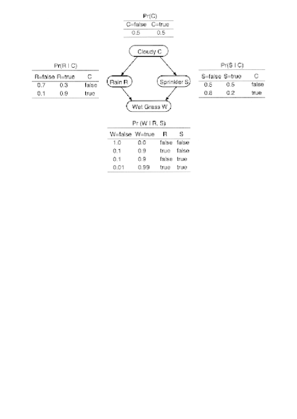
Fig. 6. Example of a well known Bayesian network describing probabilistic
dependencies among variables Cloudy (C), Sprinkler (S), Rain (R), and Wet
Grass (W). These probabilities form the basis for computing the joint proba-
bility: P(C, R, S, W) P(C) P(R|C) P(S|C) P(W|R, S), that is, the probability

of observing a combination of states assuming the specified probabilistic
dependencies among the nodes. In this example, the probability of seeing wet
grass for a cloudy sky with rain and no sprinkler on is 0.5

=

=
0.324. Not all states in the network may be known or observable at any given
time. With BNs, marginal probabilities for subsets of known states can be
obtained from the joint probability by summing over all possible combinations
of states for the unknown variables. For example, if we could not observe R or
S , we would obtain the marginal probability. In this way, the unknown vari-
ables R and S are eliminated from the distribution. Thus, we see that the like-
lihood of seeing wet grass when it is cloudy is (0.5

× 0.9 × 0.8 × 0.9

× 0.1 × 0.8 × 0.0) + (0.5 ×

0.1 × 0.2 × 0.9) + (0.5 × 0.9 × 0.8 × 0.9) + (0.5 × 0.9 × 0.2 × 0.99) = 0.4221.

for the investigators to treat non-statistical concepts, such as influence,
confounding, effect, intervention, explanation, disturbance, etc. 267
BN methods has been applied to the prediction of binding pep-
tides to HLA-A2 class I molecules. 271 Astakhov and Cherkasov (2005),
based on a data set consisting of 244 HLA-A2-binders (derived from