Prediction of floods in ungauged basins - Runoff Prediction in Ungauged Basins: Synthesis across Processes, Places and Scales - page 216

Flood frequency Flow duration Snow water equiv. 1000 of 100 years simulations

200 1 0.8

a) b) c) d)

1000

0.8

150 0.6

800

0.6

600

100 0.4

0.4

400

50 0.2

0.2

200

0 0 0 0

2 10 100 0 1 2 2 10 100 2 10 100 1000 10000

Return period (yrs) Runoff (m³/s) Return period (yrs) Return period (yrs)

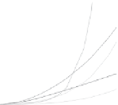
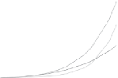
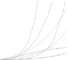
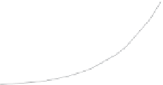
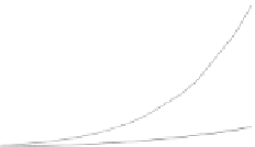
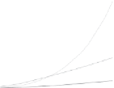
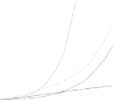
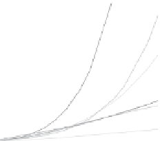
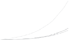
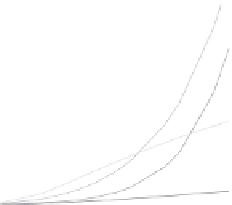
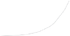
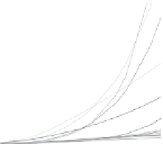
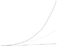
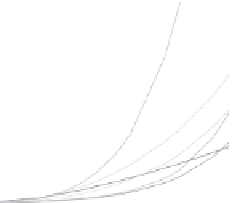
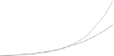
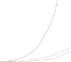
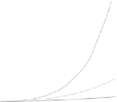
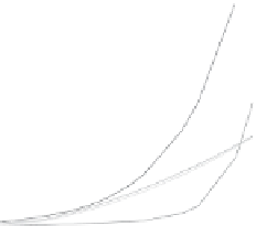
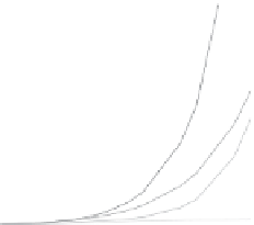
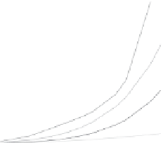
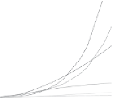
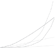
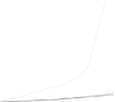
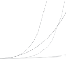
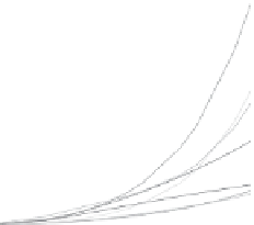
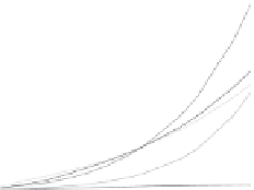
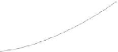
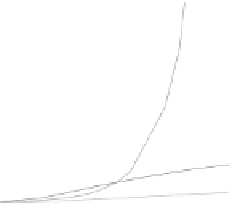
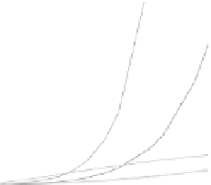
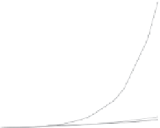
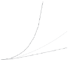
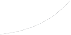
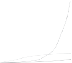
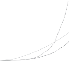
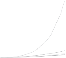
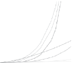
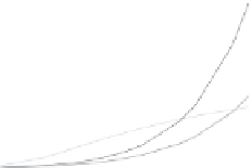
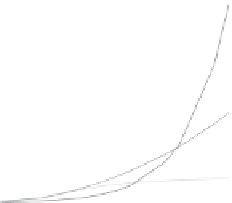
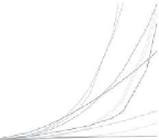
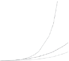
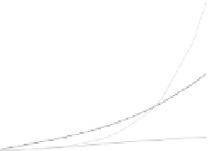
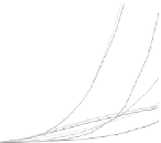
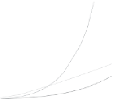
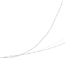
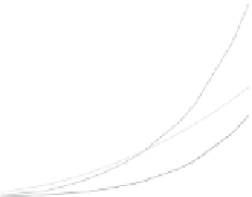
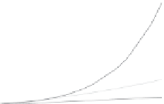
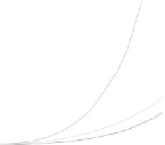
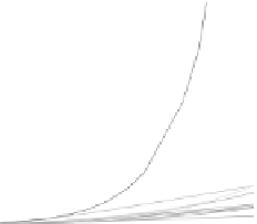
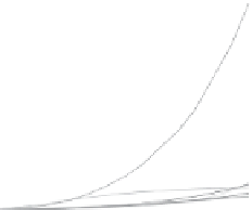
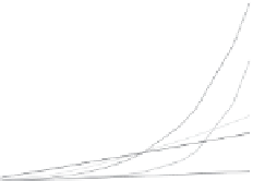
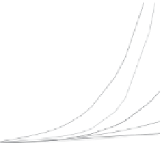
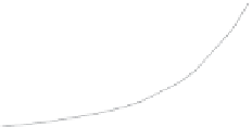
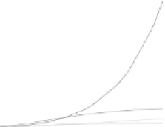
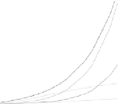
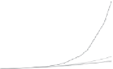
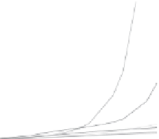
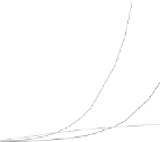
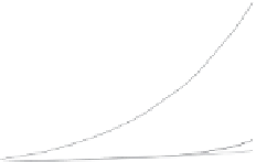
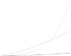
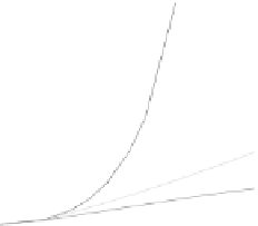
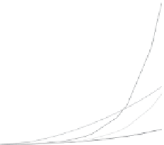
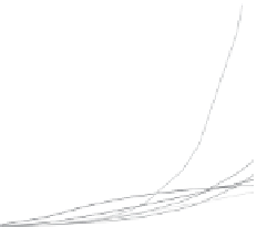
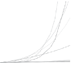
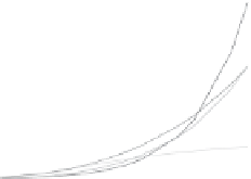
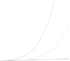
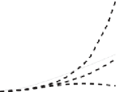
Figure 9.20. Comparison of ungauged process-based estimation and gauged statistical estimation of the flood frequency curve for the Joseful
Dul catchment in the Czech Republic. Circles refer to data or reference values, dashed lines to statistical procedures and shaded lines to
ensembles of modelled behaviours. From Blazkova and Beven ( 2002 ).

Continuous models for estimating a flood of a given
return period are usually driven by rainfall generated by a
stochastic rainfall model (Robinson and Sivapalan, 1997b ;
Menabde and Sivapalan, 2001 ; Viglione et al., 2012 ) and
the simulated runoff hydrograph is evaluated in terms of
flood peaks in the same way as an observed hydrograph.
There is therefore no issue with the mapping of the return
periods. However, other issues remain. Since the concern
is accurate reproduction of annual maximum floods with
increasing return period, there needs to be explicit recog-
nition that the model faithfully reproduces the runoff pro-
cesses that realistically could occur under extreme
conditions. Specifically, the issue is whether the model
accurately reproduces the processes associated with
changing runoff generation mechanisms and dynamics of
flood movement and inundation that could be faced under
extreme conditions. This is hard to achieve and verify,
since it is quite likely that the conditions experienced are
different from those during normal flows, and therefore
cannot be accomplished by simply calibrating against a
continuous runoff hydrograph. Information from field
visits ( Chapters 3 and 4 ) and other information about the
flow paths and local runoff processes may assist in captur-
ing the transition from normal to extreme events.
Similarly to event-based models, the model parameters
need to be estimated for the ungauged basin. Different
methods have been proposed in the literature for parameter
transfer to ungauged conditions (see Chapter 10 ). The
options are: a-priori estimation of model parameters; con-
straining model parameters by dynamic proxy data and
runoff; and transferring calibrated model parameters from
gauged catchments. The last is the most common approach
for continuous runoff models and can be obtained by
spatial proximity methods, regional calibration and down-
scaling methods, and regressions between model param-
eters and catchment characteristics. The conventional
approaches employ a two-step procedure to establish

transfer functions: gauged catchments are identified for
which calibration of model parameters is separately carried
out; then a transfer function relationship is identified,
which associates a parameter value to hydrological charac-
teristics through a regression procedure.
The calibration of continuous models to be used in flood
frequency analysis is focused on flood peaks. For example,
in Lamb and Kay ( 2004 ) the parameters are calibrated for
gauged catchments in order to minimise the difference
between the ranked simulated and observed flood peaks
and are then regionalised through multiple regressions with
catchment characteristics. They found their results for catch-
ments in Great Britain to be similar to those obtained by a
conventional statistical method. Other examples of continu-
ous modelling to estimate flood probability in ungauged
catchments include Sweden (Harlin and Kung, 1992 ), UK
(Calver et al., 1999 , 2004 ;Lamb, 2005 ), Czech Republic
(Blazkova and Beven, 2002 , 2004 ) and Austria (Rogger
et al., 2012a , b ). Blazkova and Beven ( 2002 )calibrated
model parameters for a Czech catchment treated as ungauged
with the generalised likelihood uncertainty estimation
(GLUE) methodology of Beven and Binley ( 1992 ), condi-
tioned to the statistical regional estimation of flood quantiles
for low return periods (e.g., up to 10 years), flow duration
characteristics and maximum annual snow-water equivalent.
The model was then used to estimate high return period
floods with a Monte Carlo procedure. An example of the
simulations is shown in Figure 9.20 . The figure illustrates the
enormous spread of simulations that may be encountered in
Monte Carlo simulations even though the simulations are
constrained by regional information.
So far the relative performances of the continuous simu-
lation method and regional statistical methods have not
been fully evaluated. Lamb and Kay ( 2004 ) show results
similar to the statistical procedure and Rahman et al.
( 2011b ) showworse performance. It is clear that the perform-
ance of the simulation methods very much depends on the