Prediction of floods in ungauged basins - Runoff Prediction in Ungauged Basins: Synthesis across Processes, Places and Scales - page 190

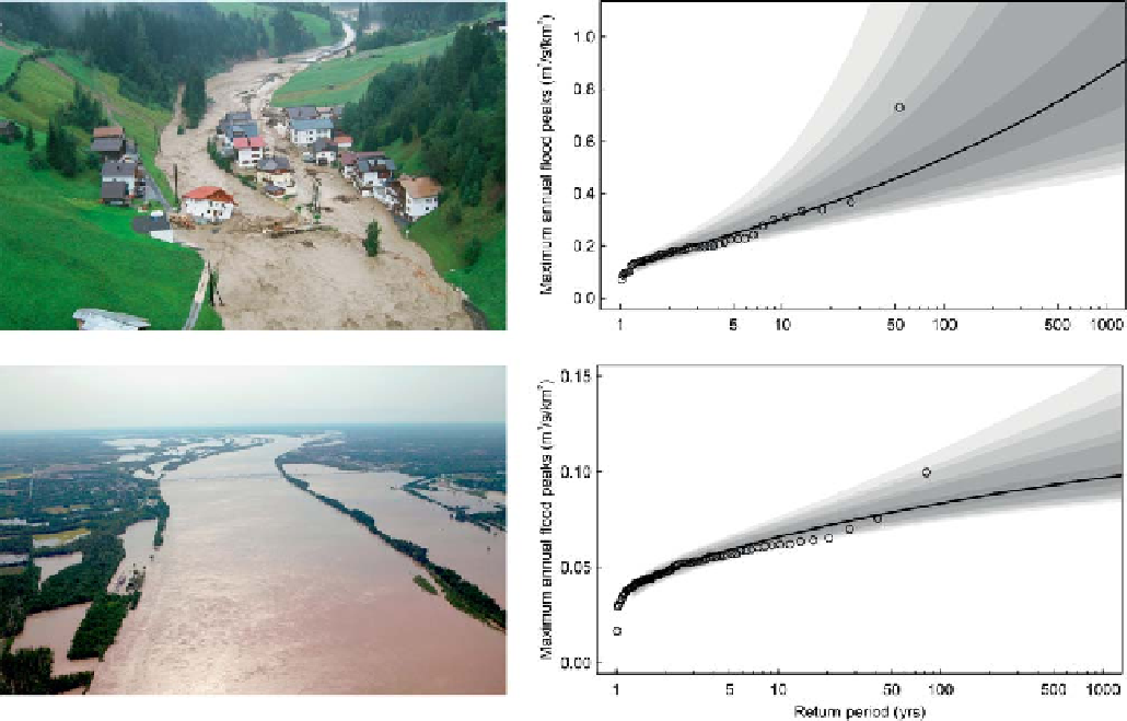
Figure 9.1. Comparative photos and flood frequency curves. (Top) 2005 flood of the Trisanna at Kappl Nederle, Austria (area 385 km 2 , median
elevation 2300 m a.s.l.); (bottom) 2011 flood of the Ohio at Metropolis, USA (area 526 000 km 2 , median elevation 84 m a.s.l.). Generalised
extreme value distribution fitted to the maximum annual floods by a Bayesian method. Grey shading represents the confidence intervals from
50% to 99.9%. Photos: (top) ASI / Land Tirol / B. H. Landeck; (bottom) B. Dodson.

the other runoff signatures discussed in this topic, in par-
ticular annual runoff ( Chapter 5 ), which reflects the aver-
age behaviour of the catchment system, and seasonal
runoff ( Chapter 6 ), which reflects the within-year variabil-
ity of precipitation, snow and soil moisture. Floods are
apparent in the flow duration curve ( Chapter 7 ) and in the
entire hydrograph ( Chapter 10 ), and they share some simi-
larities with low flows as they are both runoff extremes
( Chapter 8 ). These connections can help improve flood
predictions, and help advance predictions in general
through the improved understanding that is generated.

represented as open circles in the graph, have values
between 0.1 and 0.4 (m 3 /s)/km 2 with the exception of
one event. The August 2005 event was the highest flood
on record (shown in the picture) and had a specific
discharge of 0.73 (m 3 /s)/km 2 . In the Ohio River ( Figure
9.1 bottom) the observed specific discharges are always
lower than 0.1 (m 3 /s)/km 2 . Even the April 2011 event
(shown in picture), which was one of the most damaging
floods in the USA in the last century, only had a specific
discharge of 0.068 (m 3 /s)/km 2 . From a hydrological point
of view, it is of interest to understand why the specific
runoff peaks in the Austrian catchment are so much
higher than those in the USA catchment. In addition, the
variability of the observed peak runoff events in the
Trisanna is higher than that in the USA (coefficient of
variation 0.5 and 0.2 respectively). This translates into a
steeper flood frequency curve for the Trisanna, and a
flatter flood frequency curve for the Ohio River. It is
interesting to explore these differences in terms of the
causal processes shaping the flood frequency curves.

9.2 Floods: processes and similarity
What makes two catchments similar in terms of flood
frequencies? Figure 9.1 shows floods in two catchments
in different parts of the world along with their flood
frequency curves. In the Trisanna River in Tirol, Austria
( Figure 9.1 top), the annual maximum runoff peaks,