NANOSCALE IMAGE PROCESSING - Bio-Inspired and Nanoscale Integrated Computing - page 527

x( N - 2)

x(0) x(2) x(4)

x(1) x(3)

N /2 − Point DFT

F 1 (0) F 1 (1) F 1 (2)

N
F 1 ( )
2

- 1

F 2 (0) F 2 (1)

N

W

2 − Point

DFT

N
X ( )
2

X (0) X (1)

- 1

N N

X ( )
2

X ( ) X ( N - 1)

+ 1

2

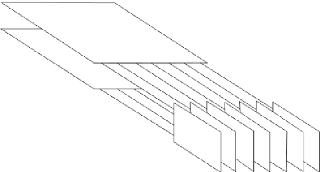
Figure 19.5. The radix-2 decimation-in-time FFT algorithm [27].

19.2.2. Implementation of the DFT and FFT
In this section, we first show how to compute DFT coefficients using a simplified
version of nanoscale spin-wave reconfigurable mesh architecture, and afterwards,
we discuss how this solution can be optimized using FFT techniques.
The DFT module consists of an N N array of input plus N output computing
nodes. In this architecture, in each row, one of the N Fourier coefficients
is computed. In other words, the kth row computes X[k] for k=0,

y , N 1.

As mentioned previously, the DFT coefficients are computed as

X ð k Þ¼ X

N 1

x ð n Þ W k N ;

0 k N

: ð 19 : 8 Þ

x ¼ 0

W N ¼ e j2 p= N

First the W N k coefficients are mapped to nodes in row k and column N,as
shown in the structure of the DFT module in Figure 19.6. The multiplication of
W N k and the inputs, x[k], is done in the processing nodes, while the summation is
performed in the spin-wave bus by employing the superposition property of the
waves.
Note that all the W N k coefficients are complex numbers. The multiplications of
the complex numbers are performed in the processing nodes as four real number
multiplications. The addition of the complex numbers on the spin-wave bus is
performed in two steps: summation of the real parts and summation of the
imaginary parts. After the multiplications are done in the processing nodes, they
send the ''real'' part of the product on the bus in the first step and the ''imaginary''