Geology Reference
In-Depth Information
Magnetic surveys are capable of locating massive sul-
phide deposits (Fig. 7.25), especially when used in con-
junction with electromagnetic methods (see Section
9.12). However, the principal target of magnetic survey-
ing is iron ore.The ratio of magnetite to haematite must
be high for the ore to produce significant anomalies, as
haematite is commonly non-magnetic (see Section 7.2).
Figure 7.26 shows total field magnetic anomalies from an
airborne survey of the Northern Middleback Range,
South Australia, in which it is seen that the haematitic
ore bodies are not associated with the major anomalies.
Figure 7.27 shows the results from an aeromagnetic sur-
vey of part of the Eyre Peninsula of South Australia
which reveal the presence of a large anomaly elongated
east-west. Subsequent ground traverses were performed
over this anomaly using both magnetic and gravity
methods (Fig. 7.28) and it was found that the magnetic
and gravity profiles exhibit coincident highs. Subse-
quent drilling on these highs revealed the presence of a
magnetite-bearing ore body at shallow depth with an
iron content of about 30%.
Gunn (1998) has reported on the location of prospec-
tive areas for hydrocarbon deposits in Australia by
aeromagnetic surveying, although it is probable that
this application is only possible in quite specific
environments.
In geotechnical and archaeological investigations,
magnetic surveys may be used to delineate zones of fault-
ing in bedrock and to locate buried metallic, man-made
features such as pipelines, old mine workings and build-
ings. Figure 7.29 shows a total magnetic field contour
map of the site of a proposed apartment block in Bristol,
England.The area had been exploited for coal in the past
and stability problems would arise from the presence of
old shafts and buried workings (Clark 1986). Lined shafts
of up to 2 m diameter were subsequently found beneath
anomalies A and D, while other isolated anomalies such
as B and C were known, or suspected, to be associated
with buried metallic objects.
(a)
(b)
100 km
(c)
(d)
(e)
(f)
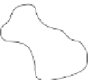
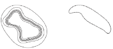
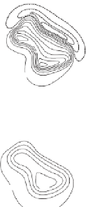
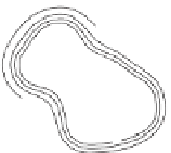
Fig. 7.23
The processing of aeromagnetic data. North direction
is from bottom to top. (a) Source body with vertical sides, 2 km
thick and a magnetization of 10 A m
-1
, inclination 60° and
declination 20°. (b) Total field magnetic anomaly of the body with
induced magnetization measured on a horizontal surface 4 km
above the body. Contour interval 250 nT. (c) Reduction to the
pole of anomaly shown in (b). Contour interval 250 nT.
(d) Anomaly shown in (b) upward continued 5 km above the
measurement surface. Contour interval 200 nT. (e) Second
vertical derivative of the anomaly shown in (b). Contour interval
50 nT km
-2
. (f ) Pseudogravity transform of anomaly shown in (b)
assuming an intensity of magnetization of 1 A m
-1
and a density
contrast of 0.1 Mg m
-3
. Contour interval 200 gu. (g) Magnitude of
maximum horizontal gradient of the pseudogravity transform
shown in (f ). Contour interval 20 gu km
-1
. (h) Locations of
maxima of data shown in (g). Note correspondence with the
actual edges of the source shown in (a). (Redrawn from Blakely &
Connard 1989.)
(g)
(h)