Geology Reference
In-Depth Information
400
200
0
km
20
200
100
Δ
g
Δ
B
0
0
-200
Magnetic North
0
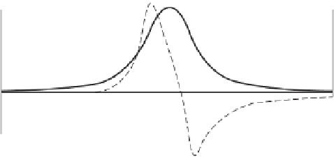
Fig. 7.14
Gravity (
D
g
) and magnetic (
D
B
)
anomalies over the same two-dimensional
body.
B
= 0.10 Mg m
-3
J
= 1 A m
-1
Δρ
10
(a)
(b)
-150
-150
km
km
-200
-200
-250
-250
-300
0
-300
0
nT
nT
10
1.6
10
0.51
20
20
-16.6
-15.6
50 km
50 km
30
30
Fig. 7.15
An example of ambiguity in magnetic interpretation.The arrows correspond to the directions of magnetization vectors, whose
magnitude is given in A m
-1
. (After Westbrook 1975.)
density is a scalar, intensity of magnetization is a vector,
and the direction of magnetization in a body closely con-
trols the shape of its magnetic anomaly. Thus bodies of
identical shape can give rise to very different magnetic
anomalies. For the above reasons magnetic anomalies
are often much less closely related to the shape of the
causative body than are gravity anomalies.
The intensity of magnetization of a rock is largely de-
pendent upon the amount, size, shape and distribution
of its contained ferrimagnetic minerals and these re-
present only a small proportion of its constituents. By
contrast, density is a bulk property. Intensity of magneti-
zation can vary by a factor of 10
6
between different rock
types, and is thus considerably more variable than den-
sity, where the range is commonly 1.50-3.50 Mg m
-3
.
Magnetic anomalies are independent of the distance
units employed. For example, the same magnitude
anomaly is produced by, say, a 3 m cube (on a metre scale)
as a 3 km cube (on a kilometre scale) with the same
magnetic properties. The same is not true of gravity
anomalies.
The problem of ambiguity in magnetic interpretation
is the same as for gravity, that is, the same inverse problem
is encountered. Thus, just as with gravity, all external
controls on the nature and form of the causative body
must be employed to reduce the ambiguity. An example
of this problem is illustrated in Fig. 7.15, which shows
two possible interpretations of a magnetic profile across
the Barbados Ridge in the eastern Caribbean. In both
cases the regional variations are attributed to the varia-
tion in depth of a 1 km thick oceanic crustal layer 2.The
high-amplitude central anomaly, however, can be ex-
plained by either the presence of a detached sliver of
oceanic crust (Fig. 7.15(a)) or a rise of metamorphosed
sediments at depth (Fig. 7.15(b)).
Much qualitative information may be derived from a
magnetic contour map. This applies especially to aero-
magnetic maps which often provide major clues as to the