Graphics Programs Reference
In-Depth Information
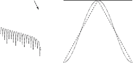
Frequency Domain
Time Domain
40
Main Lobe
Side Lobes
Rectangular
1
20
Hanning
Rectangular
0
0.8
−20
−40
0.6
Bartlett
−60
0.4
−80
−100
Hanning
0.2
−120
Bartlett
−140
0
0
0.2
0.4
0.6
0.8
1.0
0
10
20
30
40
50
60
Frequency
Time
a
b
Fig. 5.4
Spectral leakage.
a
The relative amplitude of the side lobes compared to the main
lobe is reduced by multiplying the corresponding time series with
b
a window with smooth
ends. A number of different windows with advantages and disadvantages are available
instead of using the default rectangular window, including
Bartlett
(triangular) and
Hanning
(cosinusoidal) windows. Graph generated using the function
wvtool
.
Welch (1967) (Fig. 5.5). The method includes dividing the time series into
overlapping segments, computing the power spectrum for each segment and
averaging the power spectra. The advantage of averaging spectra is obvious,
it simply improves the signal-to-noise ratio of a spectrum. The disadvantage
is a loss of resolution of the spectrum.
The Welch spectral analysis that is included in the Signal Processing
Toolbox can be applied to the synthetic data sets. The MATLAB function
periodogram(y,window,nfft,fs)
computes the power spectral den-
sity of
y(t)
. We use the default rectangular window by choosing an empty
vector
[]
for
window
. The power spectrum is computed using a FFT of
length
nfft
of 1024. We then compute the magnitude of the complex out-
put
pxx
of
periodogram
by using the function
abs
. Finally, the sampling
frequency
fs
of one is supplied to the function in order to obtain a correct
frequency scaling of the
f
-axis.
[Pxx,f] = periodogram(y,[],1024,1);
magnitude = abs(Pxx);
plot(f,magnitude),grid
xlabel('Frequency')
ylabel('Power')
title('Power Spectral Density Estimate')
The graphical output shows that there are three signifi cant peaks at the posi-