Graphics Programs Reference
In-Depth Information
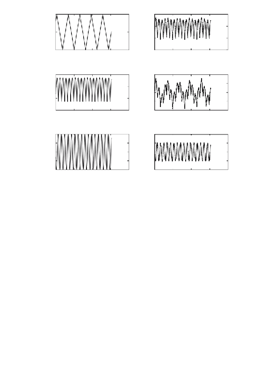
Raw Signals
Mixed Signals
0.5
0.5
0
0
−0.5
−0.5
−1
0
1000
2000
3000
4000
0
1000
2000
3000
4000
a
b
0.5
0.4
0.2
0
0
−0.5
−0.2
−1
−0.4
0
1000
2000
3000
4000
0
1000
2000
3000
4000
c
d
1
2
0.5
1
0
0
−0.5
−1
−1
−2
0
1000
2000
3000
4000
0
1000
2000
3000
4000
e
f
Fig. 9.5
Sample input for the independent component analysis. We fi rst generate three period
signals (
a
,
c
,
e
), mix the signals and add some gaussian (
b
,
d
,
f
).
x = [.1*s1 + .8*s2 + .01*randn(length(i),1),...
.4*s1 + .3*s2 + .01*randn(length(i),1),...
.1*s1 + s3 + .02*randn(length(i),1)];
subplot(3,2,2), plot(x(:,1)),
ylabel('x_1'), title('Mixed signals')
subplot(3,2,4), plot(x(:,2)), ylabel('x_2')
subplot(3,2,6), plot(x(:,3)), ylabel('x_3')
We begin with the separation of the signals using the PCA. We calculate the
principal components and the whitening matrix
W_PCA
with
[E sPCA D] = princomp(x);
The PC scores
sPCA
are the linearly separated components of the mixed
signals
x
(Fig. 9.6).