Graphics Programs Reference
In-Depth Information
plot(f,magnitude),grid
xlabel('Frequency')
ylabel('Power')
title('Power Spectral Density Estimate')
Let us increase the noise level. The gaussian noise has now a standard devia-
tion of fi ve and zero mean.
randn('seed',0);
n = 5*randn(size(y));
yn = y + n;
[Pxx,f] = periodogram(yn,[],1024,1);
magnitude = abs(Pxx);
plot(f,magnitude), grid
xlabel('Frequency')
ylabel('Power')
title('Power Spectral Density Estimate')
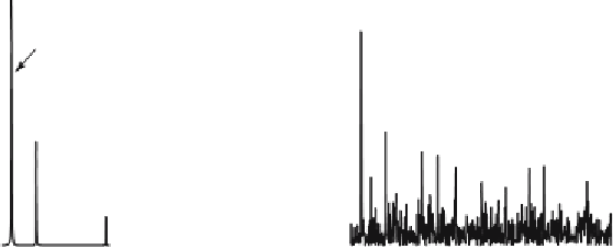
This spectrum resembles a real data spectrum in the earth sciences. The
spectral peaks now sit on a signifi cant noise fl oor. The peak of the high-
est frequency even disappears in the noise. It cannot be distinguished from
maxima which are attributed to noise. Both spectra can be compared on the
same plot (Fig. 5.6):
[Pxx,f] = periodogram(y,[],1024,1);
magnitude = abs(Pxx);
Power Spectral
Density Estimate
Power Spectral
Density Estimate
1000
1000
f
1
=0.02
800
800
f
1
=0.02
600
600
f
2
=0.07
f
2
=0.07
f
3
=0.2 ?
Noise
floor
400
400
f
3
=0.2
200
200
0
0
0.1
0.3
0.4
0.5
0.5
0
0.2
0
0.1
0.2
0.3
0.4
Frequency
Frequency
a
b
Fig. 5.6
Comparison of the Welch power spectra of the
a
noise-free and
b
noisy synthetic
signal with the periods
τ
3
=5 (
f
3
=0.2). In particular, the
peak with the highest frequency disappears in the noise fl oor and cannot be distinguished
from peaks attributed to the gaussian noise.
τ
1
=50 (
f
1
=0.02),
τ
2
=15 (
f
2
§0.07) and