Environmental Engineering Reference
In-Depth Information
measurement (Brackley, 1975; Sridharan et al., 1986). The
ability to numerically simulate the development of swelling
pressure should assist in determining the test procedure that
should be used in the laboratory. Such a simulation model
was developed by Shuai and Fredlund (1997). The model
can be used to study factors that influence the swelling pro-
cess and the development of the swelling pressure.
The swelling process involves two primary processes: the
transient water flow process and the soil volume change
(i.e., stress-deformation) process. These two processes are
interrelated and governed by the following basic equations:
(i) force equilibrium equations for the soil, (ii) constitutive
equations for unsaturated soils, and (iii) continuity equation
for the pore fluids. These equations have already been pre-
sented in Chapter 16 and will not be repeated. Relevant
equations for the uncoupled and uncoupled formulations
appear in Eqs. 16.78-16.87. Details of the theoretical for-
mulation can also be found in Shuai and Fredlund (1997).
The following assumptions are made in the derivation:
(i) the soil is isotropic, (ii) strains are infinitesimal, and
(iii) permeability with respect to the air phase is significantly
greater than permeability with respect to the water phase.
Consequently, the pore-air pressure is always equal to the
surrounding atmospheric air pressure (i.e.,
u
a
=
16.10.2 Illustration and Verification of Numerical
Swelling Pressure Model
The one-dimensional swelling process can be solved using
Eqs. 16.88 and 16.89. These equations were previously used
to simulate one-dimensional swelling and consolidation. Dif-
ferent boundary conditions need to be applied when simulat-
ing the processes associated with
free
-
swell
oedometer tests
and
constant
-
volume
oedometer tests. Laboratory tests on
compacted Regina clay are used to illustrate the simulation
of the swelling pressure tests. Specimens of Regina clay pre-
pared with a molding water content of 26% and an initial
void ratio of 0.96 were used for the numerical simulations
and verification of the theoretical formulation.
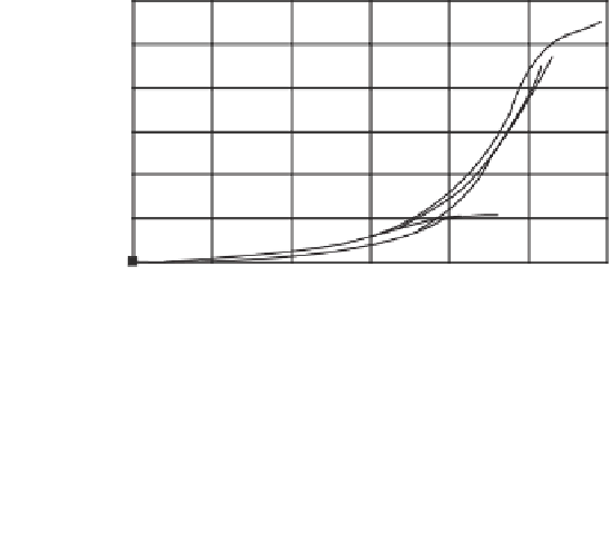
Figure 16.57 shows the measured and computed deflec-
tion versus time curves for two 100-mm-high specimens and
two 20-mm-high specimens subjected to free-swell oedome-
ter test conditions. A comparison between the computed and
measured matric suction profiles for the 100-mm-high spec-
imen subjected to free-swell oedometer test conditions is
presented in Fig. 16.58. Matric suctions were measured by
placing Whatman No. 42 filter papers between the soil lay-
ers of the specimen and measuring the water content of the
filter papers after the test. In general, the computed values
for matric suction are in good agreement with the measured
values. There are some differences between the computed
and measured matric suction profile noted during the middle
stage of the test (i.e.,
t
0). Conse-
quently, the net normal stress
(σ
u
a
)
becomes equal to the
total vertical stress
σ
and matric suction
u
a
−
−
u
w
becomes
equal to the negative pore-water pressure
u
w
. The above
assumptions allow the constitutive equations to be rewritten
in terms of the strain associated with the soil structure.
The transient water flow process is linked to the soil vol-
ume change process during the swelling process and the two
processes are solved simultaneously for the simulation of the
swelling process along a variety of stress paths.
5300 min). There are also some
differences in the matric suctions measured and predicted
in the upper portion of the specimen; however, the mea-
sured results are reasonably close to the computed matric
suctions.
Figure 16.59 shows the measured and computed vertical
stress versus elapsed time curves for two 100-mm-high
specimens and two 20-mm-high specimens subjected to
constant-volume oedometer test conditions. The measured
and computed profiles of matric suction from within the
soil specimens are presented in Fig. 16.60. The results show
good agreement between the measured and computed matric
suction values.
=
16.10.1 Specialization of Three-Dimensional Swelling
to
K
0
Loading Case
Displacements in the
x-
and
z-
directions (i.e., displacements
u
and
w,
respectively) are equal to zero for
K
0
loading.
Assuming that the pore-water pressure
u
w
and the displace-
ments do not change across the
x-
and
z-
directions, the
displacement in the
y-
direction,
v
, can be calculated. The soil
compressibility moduli
m
2
,m
1
,m
1
,
and
m
2
were defined
in Chapter 13. The soil volume change and the transient
water flow equations are simplified to the following forms:
12
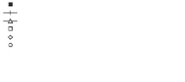
100 mm
100 mm specimen (FSSM3)
100 mm specimen (FSSM4)
100 mm specimen (computed)
20 mm specimen (FST1)
20 mm specimen (FST2)
20 mm specimen (computed)
-
-
-
-
-
10
∂
2
v
∂y
2
∂u
w
∂y
8
m
2
=−
(16.88)
6
∂
v
∂y
k
w
m
1
m
1
∂
∂t
∂
∂y
∂u
w
∂y
1
ρ
w
g
=
4
20 mm
m
2
−
∂u
w
∂t
2
m
2
·
m
1
m
1
+
(16.89)
0
0.1
1
10
100
1000
10,000 100,000
Time (min)
Equations 16.88 and 16.89 are the governing equations
that can be used to simulate the one-dimensional swelling
process (Shuai and Fredlund, 1997).
Figure 16.57
Computed and measured deflection versus time
curves for free-swell oedometer tests.


Search WWH ::

Custom Search