Environmental Engineering Reference
In-Depth Information
fill did not allow sufficient time for pore-water pressure
equilibrium. Therefore, the soil simply responded to the net
change in total stress. Second, it is assumed that the soil
approached saturation when the final pore-water pressure
was
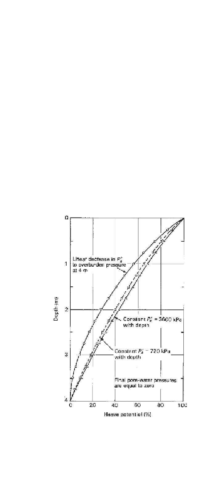
by the maximum heave in any layer. Three initial swelling
pressure profiles are assumed. The first profile assumes a
constant swelling pressure of 720 kPa throughout the 4-m
depth. The second profile assumes a constant value for the
swelling pressure of 3600 kPa throughout the 4-m depth.
The third profile assumes a linear decrease in swelling
pressure from 720 kPa to a value equal to the overburden
pressure at 4 m. All cases show that the heave potential
decreases rapidly with depth. The swelling pressure gener-
ally decreases with depth in situ, and as a result the decrease
in heave potential is of an exponential form (Fig. 14.40).
The change in water content,
w
,
can also be estimated
as the soil swells provided the initial volume-mass soil prop-
erties are known:
−
7.0 kPa. Therefore, the slope of the rebound curves
on the matric suction plane was the same as the slope on
the total stress plane. This assumption is reasonable as long
as the final pore-water pressure is relatively small.
14.5.7 Third Example of One-Dimensional Heave
Calculations
A third example illustrates the amount of heave versus depth
for a 4-m layer of expansive soil. The results show that the
largest amount of heave occurs near the ground surface.
The matric suction generally has a maximum value near the
ground surface and the overburden pressure is also lowest
near ground surface. Consequently, the ratio of the final
stress state
P
f
to the initial stress state
P
0
in Eq. 14.18
approaches its minimum value, which results in the largest
calculated heave.
Let us assume that the clay becomes wet and the
pore-water pressures go to zero throughout the deposit.
Figure 14.40 shows the distribution of heave potential
versus depth for the 4-m-thick layer. Heave potential is
defined as the heave in each layer of the profile divided
S
f
e
G
s
e
0
S
G
s
w
=
+
(14.20)
where:
S
f
=
final degree of saturation,
G
s
=
specific gravity of soil solids, and
S
=
change in degree of saturation.
The final degree of saturation can be assumed to approach
100%. Changes in void ratio,
e
, are obtained from the
heave analysis.
14.5.8 Case History (Slab-on-Grade Floor, Regina,
Saskatchewan, Canada)
In 1961, the Division of Building Research, National
Research Council, Government of Canada, monitored the
performance of a light industrial building which was con-
structed in north-central Regina. Details of the study were
presented by Yoshida et al., (1983). Instrumentation was
installed to monitor ground movements at various depths
below the slab. Water content changes were monitored
using a neutron moisture meter probe. Undisturbed samples
were taken as part of the subsurface exploration prior to the
construction of the building. Constant-volume oedometer
tests were performed on three samples, and the swelling
pressure profiles are shown in Fig. 14.41. The average
swelling index of the soil at this site was 0.09.
The owner noticed considerable cracking of the floor slab
about one year after completion of construction. Precise
level surveys showed the maximum total heave to be 106
mm. The owner had also noticed a significant increase in
water consumption (i.e., 35,000 L). It was discovered that
a leak had occurred in the hot-water line beneath the floor
slab near the location of the maximum heave. The leak was
immediately repaired.
Total heave predictions were made on the basis of the
laboratory oedometer test results. Various assumptions were
made concerning the final pore-water pressure conditions as
part of the one-dimensional heave analysis. The predicted
heave was 141mm when it was assumed that the soil had
Figure 14.40
Heave potential versus depth for various distribu-
tions of swelling pressure with depth.


Search WWH ::

Custom Search