Heat Flow Analysis for Unsaturated Soils - Unsaturated Soil Mechanics in Engineering Practice - page 512

10 6
J/m 3 / ◦ K. The volumetric heat capacity of the frozen soil is
estimated at 2 . 070

T , ° C

heat capacity of the unfrozen soil is estimated at 2 . 5 ×

− 30 − 20 − 10 0 10 20 30

0.0

10 6 J/m 3 / ◦ K. The thermal conductivity
of the unfrozen soil is estimated to be 1.3 W/m/K and the
thermal conductivity of the frozen soil is 1.55 W/m/K.
The diameter of the pipeline is 0.3 m and the top of the
pipeline is 0.3 m below ground surface. The temperature of
the ground surface is assumed to remain constant at 3.0 ◦ C.
Figure 10.28 shows the geometry of the problem along with
boundary and initial conditions. Also shown is the final auto-
matically generated mesh associated at an elapsed time of
7 days. Figure 10.29 shows the isotherms around the pipeline
corresponding to an elapsed time of 7 days. The freezing
front is on average about 0.1 m outside the pipeline.
Figure 10.30 shows the isotherms around the pipeline after
730 days. The freezing front has now extended about 0.6 m
below the invert of the pipe and about 0.1 m above the pipe.
The soil and the pipeline appear to have reached a steady-
state condition after an elapsed time of 730 days. The slope
of the SFCC, m i 2 , no longer has any influence on the solution
after 730 days.
The above heat flow example problem has involved the use
of constant specific heat soil properties. The thermal conduc-
tivity is also assumed to have constant values in the unfrozen
and frozen states. There is a change in thermal conductivity
as the soil changes phases from liquid to ice, and this change
is taken into account in the analysis.
The thermal conductivity and volumetric heat capacity
properties do not need to be changed during the heat
flow process unless there is a change in the volume-mass
properties of the soil.

Asphalt
Layer 1

×

0.5

Layer 2

1.0

1.5

Subgrade

2.0

2.5

3.0

Figure 10.25 Temperature isotherms below highway surface for
each month of the year (from Cote, 2009; Colloquium address)

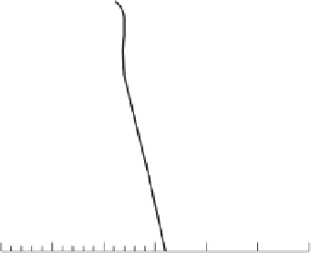
a temperature of 3 ◦ C. Figure 10.26 shows the unfrozen water
content versus temperature graph, referred to as the SFCC.
The slope of the SFCC is given the symbol m i 2 . The SFCC
forms a continuous function with respect to temperature. Small
temperature change steps must be used for the soil-freezing
curve in order to ensure convergence to the correct solution.
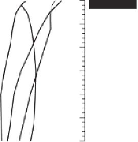
Figure 10.27 shows a plot of thermal conductivity versus
temperature for the soil surrounding the pipeline. The vol-
umetric water content of the soil is 37.7%. The volumetric

100

80

60

10.10 TWO-DIMENSIONAL HEAT FLOW
EXAMPLE WITH SURFACE TEMPERATURES
ABOVE AND BELOW FREEZING

40

20

0

The next example problem has a two-dimensional geome-
try and involves consideration of the latent heat of fusion
associated with the freezing and thawing of soil. The results
were published by Harlan and Nixon (1978) and have been
used as a benchmark solution.

− 2 − 1 0 1 2

Temperature, °C

Figure 10.26 SFCC for the soil.

1.6

10.10.1 Description of Two-Dimensional Heat
Flow Problem
Harlan and Nixon (1978) performed a steady-state analysis
involving the heat transfer between two adjacent areas with
a ground surface temperature of

1.5

1.4

4 ◦ C on the left side and +

5 ◦ C on the right side, as shown in Fig. 10.31. The thermal
conductivity of the soil was estimated to be 1.0 W/m/K.
The computer simulation was set up as two adjacent semi-
infinite regions. One region was subjected to a surface tem-
perature of

1.3

−

1.2

− 2 − 1 0 1 2

Temperature, °C

4 ◦ C while the other surface had a temper- +

5 ◦ C. The soil temperatures were computed for

ature of −

Figure 10.27 Thermal conductivity of unfrozen and frozen soil.