Environmental Engineering Reference
In-Depth Information
Third, it must be possible to measure or estimate the ther-
mal soil properties and other soil properties relevant to the
problem being solved.
Fourth, boundary conditions must be applied to the bound-
aries of the geometry. Initial conditions also need to be estab-
lished when modeling situations where the partial differential
equation is time dependent. Many geothermal analyses are
not highly nonlinear, and as a result it is quite straightfor-
ward to assess initial or starting conditions when analyzing a
transient heat flow problem. It is generally advisable to first
perform a steady-state analysis, even when a transient analy-
sis is required. Heat flow problems often involve performing
numerous transient-type analyses to capture the sensitivity
associated with changing a number of variables related to the
problem at hand.
Fifth, the numerical solutions should be performed and each
set of results studied from the standpoint of reasonableness.
There are many potential sources of error when undertaking
numerical modeling studies, and it is important that the com-
puter output be properly interpreted. Most studies involve the
use of a series of analyses (i.e., a parametric or sensitivity
analysis) in order to ascertain the range of results that might
be anticipated in situ.
40
35
30
25
20
15
10
5
0
0
50
100
150
200
250
300
350
400
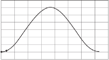
Days of the year starting at January 1
Figure 10.24
Sinusoidal variation of temperature throughout one
year.
with the graph in Fig. 10.24. The temperature throughout
365 days can be written in equation form as follows:
15 sin
π
2
+
2
πt
365
T
=
20
+
−
(10.75)
where:
temperature,
◦
C, and
T
=
t
=
time in days from January 1.
10.8 ONE-DIMENSIONAL HEAT FLOW
IN UNFROZEN AND FROZEN SOILS
The highest temperature occurs in July and the coldest
temperature occurs in January.
The first heat flow problem illustrates the solution of a tran-
sient one-dimensional geometry where the soil is unfrozen.
The initial temperature is assumed to be constant with depth,
and it is assumed that a sinusoidal temperature variation is
imposed at the ground surface over a period of one year.
The temperature profile with depth is plotted every 2 weeks
of the year.
10.8.2 Solutions of Partial Differential Heat
Flow Equation
The heat flow problem requires the solution of the partial dif-
ferential equation 10.21. The finite element mesh generated for
the solution of this problem consists of a series of nodes that are
almost equally distributed with depth. Figure 10.25 shows the
temperature isotherms with time (Cote, 2009). The isotherms
have a bell shape with the highest variations at ground surface
and virtually no change in temperature at a depth of 2.5 m.
10.8.1 Description of One-Dimensional Heat Flow
Let us consider the case where the soil profile is unfrozen
and the initial temperature is constant with depth at 15
◦
C.
The geometry consists of a column of soil 5 m high. The
ground surface is level and the geometry is one dimen-
sional. The upper meter of soil is somewhat different from
the underlying soil. Therefore, different thermal properties
are input for the zone above and below the 1-m depth.
It is necessary to input both the thermal conductivity and the
heat capacity properties for the soil since the problem under
consideration is transient in nature. The thermal conductivity
in the upper meter of soil is 1.1 W/m/K. The remaining soil
profile has a thermal conductivity of 1.9 W/m/K. The volu-
metric heat capacity of the soil in the upper meter is 2
10.9 TWO-DIMENSIONAL HEAT FLOW
EXAMPLE INVOLVING CHILLED PIPELINE
Coutts and Konrad (1994) presented an example conductive
heat flow problem that is common to the pipeline industry.
The example considers the transfer of oil or gas through a
pipeline from a northern cold region to a warmer southern
region. It is assumed that the fluid in the pipeline is chilled to
avoid thawing of the permafrost terrain. A problem may be
encountered when the pipeline passes through discontinuous
permafrost or when the terrain is not frozen.
10
6
J/m
3
/K and the remaining soil profile has a volumetric heat
capacity of 2
.
7
×
10.9.1 Description of Soil Freezing around Pipeline
Consider the case of a pipeline where the inside fluid has a
temperature of
10
6
J/m
3
/K.
The temperature imposed at the ground surface varies
from a low of
×
5
◦
C to a high of
35
◦
C, in accordance
2
◦
C. The pipeline is embedded in a soil with
+
+
−


Search WWH ::

Custom Search