Solving Saturated/Unsaturated Water Flow Problems - Unsaturated Soil Mechanics in Engineering Practice - page 429

and in the numerical simulation. The results of pore-water
pressure measurements can be compared with the computed
results from a numerical model. Close agreement has been
observed between pore-water pressure measurements and
the results of an unsteady-state finite element analysis.
An initial steady-state condition was assumed with the
water table located at a height of 0.3 m from the toe of the
slope. At an elapsed time taken as zero, a constant infiltration
rate of 2 . 1

10 − 4 m/s was applied to the top portion of the
hill slope. The development of the groundwater table from
its initial steady-state condition (i.e., at time equal to zero)
to an elapsed time of 100 s is shown in Fig. 8.64. The water
level at the toe of the slope and the infiltration rate at the top
of the slope were assumed to remain constant throughout
the transient process. No flow boundary conditions were
assumed along the remainder of the slope boundaries.
The seepage flow pattern and the development of the
equipotential lines within the slope continued to change
with elapsed time. The finite element mesh was also auto-
matically refined as necessary, internal to the analysis. The
equipotential lines and the phreatic line corresponding to an
elapsed time of 200 s are shown in Fig. 8.65. The results for
an elapsed time of 220 s are shown in shown in Fig. 8.66.
The results show a gradual rise in the lower phreatic water
surface and a gradual change in the equipotential lines. At
the start of the infiltration process, water infiltrates vertically
toward the impeding layer. As the infiltration of water
continues, water moves through the impeding layer, causing
the groundwater table to rise. After 240 s a perched water
table develops on the impeding layer and moves toward the
face of the slope (see Fig. 8.67). After 260 s a wedge-shaped
unsaturated zone is formed, and the perched water table
moves toward the edge of the slope, as shown in Fig. 8.68.
Now, two seepage faces began to develop. One seepage
face is near the toe of the slope and the other seepage face
develops at the top of the impeding layer. In other words, the
presence of the impeding layer results in a complex configura-
tion for the groundwater table and the position of the equipo-
tential lines. A steady-state condition is established after about
280 s. The steady-state results are shown in Fig. 8.69. There
is close agreement between the results of the physical model
measurements (Rulon and Freeze, 1985) and the numerical
model results. The positions of the developed water table, the
seepage faces, and pore-water pressures are similar.
The finite element numerical analyses presented for the
three example problems have illustrated the way in which
unsteady-state modeling can be performed for saturated-
unsaturated flow problems. The application of a saturated
flow model to each of these problems would be virtually
impossible to undertake. However, the use of a combined
saturated-unsaturated flow is quite straightforward. The flow
systems that developed throughout the unsaturated soil sys-
tem can be complex, depending upon the contrast in the
coefficients of permeability and the water storage modulus
for the different soils.

×

Figure 8.61 Geometry and boundary conditions for an example
involving layered soils in a hillslope.

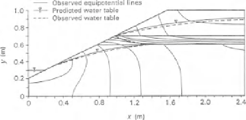
shown in Fig. 8.61. The physical model was instrumented
with pore-water pressure measuring devices. The slope con-
sisted of medium sand with a horizontal layer of fine-grained
sand. The fine sand had a lower coefficient of permeabil-
ity than the medium-grained sand. The intent was to study
whether the fine sand layer would impede water flow and
create a seepage face on the slope. The steady-state results
from the experimental measurements are shown in Fig. 8.62.
The steady-state equipotential lines and the phreatic water
surface are presented. The experimental study forms a valu-
able benchmark problem against which numerical models
can be tested.
The soil properties of the materials involved are shown
in Fig. 8.63. The two sand materials are assumed to have
the same SWCCs (Fig. 8.63a); however, the saturated coef-
ficients of permeability for the two sand materials were
different (Fig. 8.63b). The saturated coefficient of perme-
ability for the medium sand was 1 . 4 10 − 3 m/s and the

fine sands had a saturated coefficient of permeability of
5 . 5

×

10 − 5 m/s (Rulon and Freeze, 1985). The water stor-
age function for both sands was obtained by differentiating
the volumetric SWCC and the result is shown in Fig. 8.63c.
The constant rate of infiltration of 2 . 1

×

10 − 4 m/s was
applied at the top of the hill slope in the experimental model

×

Figure 8.62 Comparison of observed water table and pore-water
pressures in experimental tank with that predicted using Neu-
mann model under steady-state conditions (from Rulon and Freeze,
1985).