Solving Saturated/Unsaturated Water Flow Problems - Unsaturated Soil Mechanics in Engineering Practice - page 383

10 − 4

10 − 5

10 − 6

10 − 7

Permeability versus suction

10 − 8

Field depth 0 - 0.15 (m),
k s = 4.1 x 10 − 5 (m/s)
Field depth 0.30 - 0.45 (m),
k s = 3.6 x 10 − 5 (m/s)

10 − 9

Field depth 0.60 - 0.90 (m),
k s = 4.8 x 10 − 5 (m/s)

10 − 10

10 − 11

0 . 1 1 0 1 0 0

Matric suction ( u a - u w ), kPa

Figure 8.7 Plot of measured permeability data on Lakeland fine sand to show water coefficient
of permeability as function of soil suction.

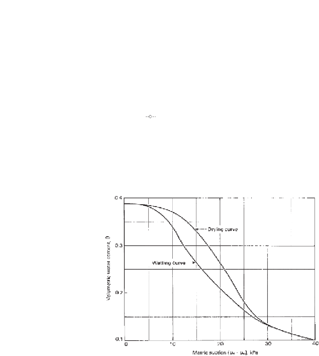
Figure 8.8 SWCC of fine tailings sand (after Gonzalez and Adams, 1980).

function k w (θ) i can also be performed for the wetting curve.
The k w (θ) i calculations should proceed from low to high
matric suction values for both the wetting and drying curves.
The water coefficients of permeability k w are computed as
a function of volumetric water content θ . It is also possible
to plot the data shown in Fig. 8.10 in the more conventional
form used for the permeability function (i.e., logarithm of
permeability versus logarithm of soil suction). Figure 8.11

shows the measured data from Gonzalez and Adams (1980)
plotted along with the computed values for the coefficient
of permeability.

8.2.4.2 Burdine Model (1953)
Several statistical models have been proposed which make
use of the Childs and Collis-George (1950) visualization
of water flow through an unsaturated soil. Examples of