Environmental Engineering Reference
In-Depth Information
where:
f
3
is added to control the transition at the air-
entry value, and
f
6
is added to control
=
w
s
gravimetric water content at soil suction of
1 kPa and
the transition at
the
residual soil suction.
S
1
,S
2
,S
3
=
slopes of the three parts of the SWCC.
The following equation can be used to represent the func-
tions
f
1
and
f
4
:
An arbitrary starting reference point for the
w
1
(ψ)
equation
is the water content corresponding to 1 kPa. Equation 5.64
can be modified so that reference suctions other than 1 kPa
are preferred:
s
n
1
f(s,s
1
)
=
(5.68)
s
n
1
s
n
+
S
2
log
ψ
ψ
aev
where:
s, s
1
,
and
n
=
S
3
log
(
10
6
)
w
2
(ψ)
=
w
aev
−
=
three arbitrary variables.
+
(S
2
−
S
3
)
log
(ψ
r
)
−
S
2
log
(ψ)
(5.65)
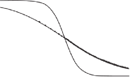
10 and varying
n
values (i.e.,
Plots of Eq. 5.68 with
s
1
=
n
1, 4, and 10) are shown in Fig. 5.55. Function
f
3
controls the transition at the air-entry value of the SWCC.
Function
f
3
can be obtained by differentiating function
f
1
on a logarithmic scale:
=
where:
w
aev
=
gravimetric water content at the air-entry value,
ψ
aev
=
soil suction at the air-entry value of the soil,
d
[
f
1
(s)
]
log
(s)
S
2
=
slope of the SWCC for the portion between the air-
entry value and the residual soil suction, and
f
3
(s)
=
α
(5.69)
S
3
=
slope of the portion beyond the residual soil suction,
where:
α
and
=
a scaling factor.
S
3
log
10
6
ψ
Function
f
6
can be obtained in a similar manner. Substi-
tuting Eqs. 5.64, 5.65, 5.66, 5.68, and 5.69 into Eq. 5.67
yields the following SWCC equation containing the slopes
of three parts of the SWCC:
w
3
(ψ)
=
(5.66)
A mathematical technique can be used to connect the
above three sloping line equations into a single SWCC
equation. A function
f
can be used to connect any two
straight lines. The function varies between 0 and 1 with an
inflection point at the intersection of the two straight lines.
This technique has been implicitly used in some SWCC
equations. A general form of the combined functions for
the SWCC-fitting equation is as follow:
⎡
S
1
)
log
ψ
ψ
aev
⎤
ln
(
10
)
2
t
1
A(ψ)
×
(S
2
−
−
⎣
⎦
A(ψ)
]
S
2
)
log
ψ
ψ
r
w
(ψ)
=
[1
−
+
(S
3
−
B(ψ))
ln
(
10
)
2
t
2
−
(
1
−
w
(ψ)
=
[
w
1
(ψ)f
1
(ψ, ψ
aev
)
+
w
2
(ψ)f
2
(ψ, ψ
aev
)
S
3
log
10
6
ψ
+
f
3
(ψ, ψ
aev
)
]
f
4
(ψ, ψ
r
)
×
B(ψ)
+
(5.70)
+
w
3
(ψ)f
5
(ψ, ψ
r
)
+
f
6
(ψ, ψ
r
)
(5.67)
where:
1
0.9
n
= 1
n
= 4
n
= 10
ψ
=
soil suction and
0.8
f
1
,f
2
,f
3
,f
4
function that must satisfy the following
conditions:
f
1
is increased to 1 when
ψ
is decreased from
ψ
aev
to 0,
f
1
is decreased to 0 when
ψ
is increased from
ψ
aev
to
=
0.7
0.6
0.5
0.4
0.3
+∞
,
0.2
f
2
=
f
1
,
f
4
is increased to 1 when
ψ
is decreased from
ψ
r
to 0,
f
4
is decreased to 0 when
ψ
is increased from
ψ
r
to
1
−
0.1
0
1
10
100
Log s
+∞
,
Figure 5.55
Plots of meaningful parameter SWCC equation used
to represent functions
f
1
and
f
4
(after Pham, 2005).
f
5
=
1
−
f
4
,


Search WWH ::

Custom Search