Environmental Engineering Reference
In-Depth Information
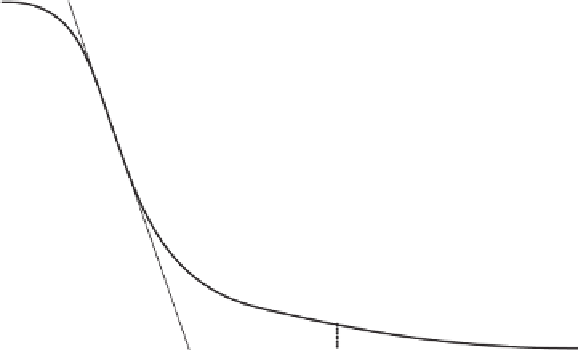
The slope
s
of the tangent
line can be calculated as
of the squared deviations of the measured data from the
calculated data) can then be minimized with respect to the
three parameters
a
f
,n
f
, and
m
f
:
follows:
θ
i
log
(ψ
p
/ψ
i
)
s
=
(5.59)
M
θ(ψ
i
,a
f
,m
f
,n
f
)
]
2
O(a
f
,m
f
,n
f
)
=
[
θ
i
−
(5.60)
where:
i
=
1
ψ
p
=
suction at intercept of the tangent line on the semilog
plot and the zero-water-content line (Fig. 5.32) and
where:
ψ
i
=
suction at inflection point on the SWCC.
O(a
f
,n
f
,m
f
)
=
objective function,
M
=
total number of measurements, and
The graphical procedure provides an approximation of
each of the fitting parameters. To obtain a closer fit to
experimental data, the three parameters (
a
f
,n
f
,
and
m
f
)
in
Eq. 5.54 can be determined using a least-squares regression
method. When performing the best-fit regression analysis,
reasonable initial values should be selected for each of the
three parameters. The following objective function (i.e., sum
θ
i
,ψ
i
=
measured values.
The best-fit regression analysis is a nonlinear minimiza-
tion process. A curve-fitting utility can be used based on
Eqs. 5.53 and 5.60 along with a quasi-Newton method.
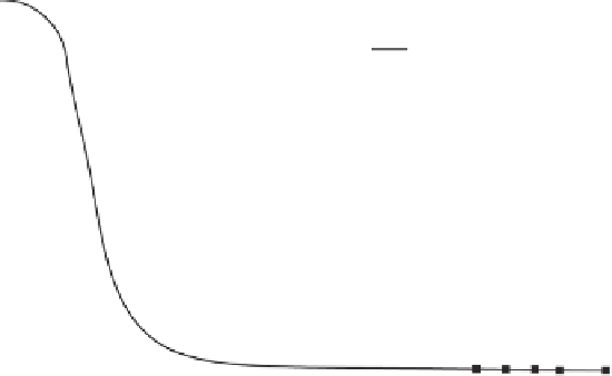
Best-fit curves for tailings sand, silt, and clay are shown in
Figs. 5.33-5.35. The regression analyses show that Eq. 5.53
θ
s
Inflection point
θ
i
(ψ
i
,
θ
i
)
θ
i
Slope =
log (
ψ
p
/
θ
i
)
(ψ
r
,
θ
r
)
θ
r
0
ψ
i
ψ
p
ψ
r
10
6
1
1000
10,000
100,000
Soil suction, kPa
Figure 5.32
Graphical estimation of four SWCC soil fitting parameters
(a
f
,n
f
,m
f
,
and
ψ
r
)
.
100
Best-fit curve
Experimental data
80
60
a
= 0.952
n
= 2.531
m
= 1.525
ψ
r
= 3000
40
20
0
10
6
0.1
1
10
100
1000
10,000
100,000
Soil suction, kPa
Figure 5.33
Best-fit Fredlund and Xing (1994) equation applied to experimental data on sand.


Search WWH ::

Custom Search