Information Technology Reference
In-Depth Information
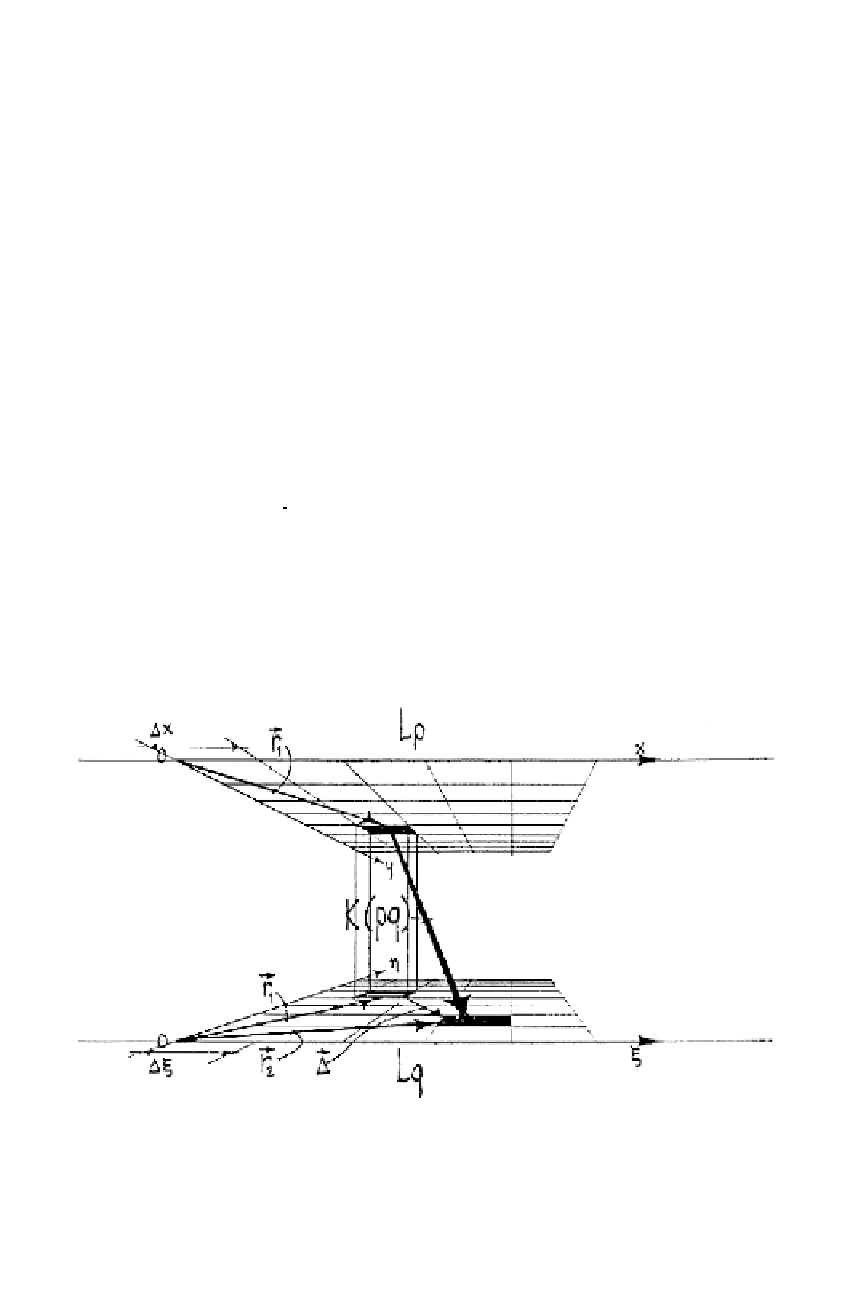
4.5. Action Networks of Discrete, Localized Elements
After these general remarks we introduce more stringent geometrical con-
straints. We now assume that elements
e
ki
are not only traceable to a certain
layer
L
k
, but also that each element within one layer can be localized as to
its precise position in this layer (see fig. 24). We first consider only action
phenomena between elements of two adjacent layers
L
i
and
L
i
+1
, which, for
simplicity, we may call
L
p
and
L
q
. We subdivide each layer into lattice ele-
ments with appropriate dimensions D
x
, D
y
, D
z
, and Dx, Dh, Dz in
L
p
and
L
q
respectively, so as to be able to accommodate in each lattice element pre-
cisely one element
e
pi
and
e
qj
respectively. For simplicity we shall assume
the corresponding lattice dimensions in both layers to be alike D
x
=Dx, etc.,
because first, it does not infringe on the generality of the remarks we wish
to make and, if there is indication to the contrary, it is not difficult to match
the metric of the two layers
L
p
and
L
q
by appropriate transformations.
We are now in a position to label each element in layers
L
p
and
L
q
accord-
ing to the coordinates of the lattice element in which it resides. Let
p
and
q
represent the coordinate triple that locates the lattice elements in the
respective layers. We have:
[
]
=◊
[
]
pxyz
,,
x
DDD
DD D
xy
,
◊
yz
,
◊
z
,
(81)
[
]
=◊
[
]
quvw
,,
u
x
,
v
◊
h z
,
w
◊
,
where
x
,
y
,
z
,
u
,
v
,
w
are integers 0, ±1, ±1,....It is clear that for one-
dimensional or two-dimensional layers the definitions for
p
and
q
boil
down to
p
[
x
],
q
[
u
], and
p
[
x
,
y
],
q
[
u
,
v
] respectively. And it is also clear that
FIGURE 24. Geometry in an action network.
Search WWH ::

Custom Search