Radar Cross Section (RCS) - MATLAB Simulations for Radar Systems Design - page 552

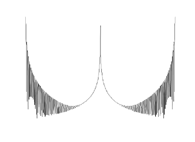
As an example, consider a circular cylinder with two perfectly conducting
circular flat plates on both ends. Assume linear polarization and let
and . The backscattered RCS for this object versus aspect angle is
shown in Fig. 11.56. Note that at aspect angles close to and the RCS
is mainly dominated by the circular plate, while at aspect angles close to nor-
mal incidence, the RCS is dominated by the cylinder broadside specular return.
The reader can reproduced this plot using the MATLAB program
Ðrcs_cyliner_complex.mÑ given in Listing 11.19 in Section 11.9.

H = 1 m

r = 0.125 m

0° 180°

30

20

10

0

-10

-20

-30

-40

-50

0 20 40 60 80 100 120 140 160 180

Aspect angle - degrees

Figure 11.56. Backscattered RCS for a cylinder with flat plates.

11.8. RCS Fluctuations and Statistical Models

In most practical radar systems there is relative motion between the radar
and an observed target. Therefore, the RCS measured by the radar fluctuates
over a period of time as a function of frequency and the target aspect angle.
This observed RCS is referred to as the radar dynamic cross section. Up to this
point, all RCS formulas discussed in this chapter assumed a stationary target,
where in this case, the backscattered RCS is often called static RCS.

Dynamic RCS may fluctuate in amplitude and/or in phase. Phase fluctuation
is called glint, while amplitude fluctuation is called scintillation. Glint causes
the far field backscattered wavefronts from a target to be non-planar. For most