Graphics Programs Reference
In-Depth Information
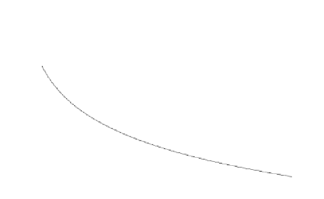
single pulse
94 pulse CI
40
30
20
10
0
-10
1
2
3
4
5
6
7
8
9
10
11
12
Detection range - Km
Figure 1.19. SNR versus detection range, using parameters from example.
Non-coherent Integration case:
Start with Eq. (1.87) with
and
,
(
SNR
)
NCI
=
10
dB
n
P
=
94
1(
2
4 4
2
10
2 4
10
94
(
SNR
)
1
=
---------------
+
-----------------
+
------
=
0.38366
⇒
4.16
dB
×
×
Therefore, the single pulse SNR when 94 pulses are integrated non-coher-
ently is -4.16dB. You can verify this result by using Eq. (1.86). The integration
loss
is calculated using Eq. (1.85). It is
L
NCI
1
+
0.38366
0.38366
L
NCI
=
----------------------------
=
3 . 6 0 6 5
⇒
5 . 5 7 1
dB
Therefore, the net non-coherent integration gain is
10
×
log
9()
5.571
=
14.16
dB
⇒
26.06422
and, consequently, the maximum detection range is
)
14
⁄
R
NCI
=
2.245
×
(
26.06422
=
5.073
Km
n
P
=
94
This means that using 94 pulses integrated non-coherently at 5.073 Km where
each pulse has SNR of -4.16dB provides the same detection criterion as using a
using the MATLAB program Ðfig1_19.mÑ.


Search WWH ::

Custom Search