The Radar Ambiguity Function - MATLAB Simulations for Radar Systems Design - page 195

The up-chirp ambiguity function cut along the time delay axis τ is

2

τ
τ'

   

sin πµττ'1 – -----

   

τ
τ'

 

) 2

------------------------------------------------

χτ0 ( ; = 1 – ----- τ ' ≤

(4.20)

 

τ
τ'

 

πµττ'1 – -----

 

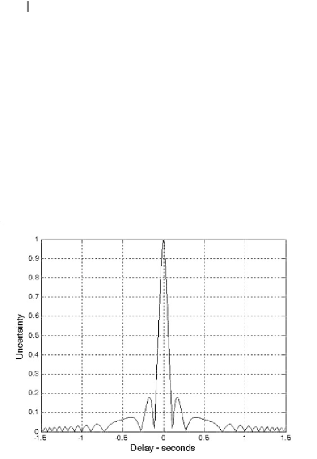
Fig. 4.6 shows a plot for a cut in the uncertainty function corresponding to
Eq. (4.20). Note that the LFM ambiguity function cut along the Doppler fre-
quency axis is similar to that of the single pulse. This should not be surprising
since the pulse shape has not changed (we only added frequency modulation).
However, the cut along the time delay axis changes significantly. It is now
much narrower compared to the unmodulated pulse cut. In this case, the first
null occurs at

τ n 1 ≈ 1 ⁄ B

(4.21)

which indicates that the effective pulsewidth (compressed pulsewidth) of the
matched filter output is completely determined by the radar bandwidth. It fol-
lows that the LFM ambiguity function cut along the time delay axis is narrower
than that of the unmodulated pulse by a factor

τ′ = 1 Figure 4.6. Zero Doppler uncertainty of an LFM pulse ( ,

). This plot can be reproduced using MATLAB
program Ðfig4_6.mÑ given in Listing 4.6 in Section 4.6.

b = 20