Graphics Programs Reference
In-Depth Information
Fresnel integrals are approximated by
1
π
x
π
C
()
1
---
x
2
≈
---
+
------
sin
;
x
»
1
(3.44)
S
()
1
π
1
π
x
---
x
2
---
≈
------
cos
;
x
»
1
(3.45)
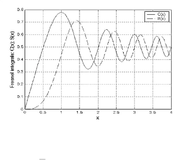
Note that and . Fig. 3.7 shows a plot of both
and for . This figure can be reproduced using MATLAB
program
Ðfig3_7.mÑ
given in Listing 3.1 in Section 3.12.
Cx
()
C
()
=
Sx
()
S
()
=
C
()
S
() 0
≤≤
x
4.0
Figure 3.7. Fresnel integrals.
Using Eqs. (3.42) and (3.43) into (3.39) and performing the integration yield
[
Cx
()
Cx
()
+
]
+
2
jSx
()
Sx
()
[
+
]
j
ω
2
S
() τ
1
B
τ
⁄
(
4π
B
)
--------------------------------------------------------------------------------------
=
------
e
(3.46)
Fig. 3.8
shows typical plots for the LFM real part, imaginary part, and ampli-
tude spectrum. The square-like spectrum shown in Fig. 3.8c is widely known
as the Fresnel spectrum. This figure can be reproduced using MATLAB pro-
gram
Ðfig3_8.mÑ
, given in Listing 3.2 in Section 3.12.
A MATLAB GUI (see Fig. 3.8d) was developed to input LFM data and dis-
play outputs as shown in Fig. 3.8. It is called
ÐLFM_gui.mÑ.
Its inputs are the
uncompressed pulsewidth and the chirp bandwidth.


Search WWH ::

Custom Search