Geology Reference
In-Depth Information
(a)
3
2
1
0.20
0.40 0.60
0.80
1.00
1.20
1.40 1.60
1.80
n/n_cal
(b)
160
meas
140
1
120
2
100
3
80
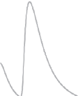
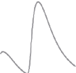
Fig. 3.2
(a) Sensitivity analysis of LISEM:
relative changes in Manning's
n
(
x
-axis)
and
K
sat
(
y
-axis) in steps of 0.2 around the
calibrated values (1.0, 1.0) and resulting
total discharge for a rainstorm event in the
Ganspoel catchment in Belgium. Legend:
white
60
40
0 m
3
total discharge.
The black isoline shows the combinations
that give the measured discharge of 253 m
3
.
(b) Simulated hydrographs for points 1, 2 and
3 in Fig. 3.2a, and the measured hydrograph
(dotted line).
=
2300 m
3
, black
=
20
0
0
50
100
150
200
t (min)
methods is that not only the observed values can
be included in the analysis, but also their uncer-
tainty. An example of this is the PEST (Parameter
Estimation) system, which can be used as a shell
coupled to virtually any model (Doherty, 2005).
Maneta
et al
. (2007) used their own model to simu-
late the discharge over a period of two months of a
small ephemeral stream in central Spain from a