Geology Reference
In-Depth Information
10
1
m
n
-
SL
(18.2)
µ
where
L
is the distance down the slope from
interfluve at the top of the slope, so that for a unit
width slope
A
8
m
n
-
1
a
is
normally in the range 0.4 to 0.8, and Equation
(18.2) shows how
a
is dependent on the physics of
the erosion process. Equation (18.2) provides a
relationship that allows design of rehabilitated
slopes that are geomorphologically stable.
To explore the implications of Equation (18.2)
using LEM simulations, Hancock
et al
. (2003)
explored the relative merits of a range of concave
slopes as batters to several above-ground con-
structed landforms at a mine site. They fitted
Equation (18.2) to natural landforms around
the mine site and found a value of
a
=
L
. For natural slopes
=
6
4
2
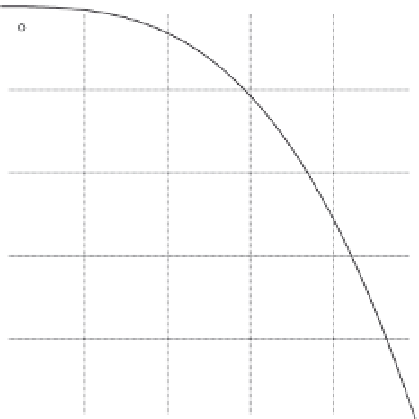
Planar slope
Concave up slope
Concave down slope
0
0
20
40
60
80
100
Hillslope distance (m)
0.35. They
also determined
m
and
n
in Equation (18.1) by cali-
brating the equation to rainfall runoff erosion simu-
lator data to yield respective values of 2.53 and 2.67
for site 1, and 1.11 and 1.5 for site 2. The data from
site 1 imply
a
=
Fig. 18.6
Three hillslope longitudinal profiles with
concavities ranging over that observed in nature.
The concavities of these slopes (Equation (18.2) ) are:
(a) concave down slope,
a
=
− 1; (b) planar slope,
0.08. The
main difference between the two sites was in the
type of waste material. Hancock
et al
. then carried
out a series of LEM simulations using the SIBERIA
LEM to compare the predicted erosion rates in t
ha
−1
. Two sets of comparison profiles were created.
The first had the concavity implied by the erosion
data for site 1 (i.e.
a
=
0.57 and from site 2
a
=
a
=
0.0; and (c) concave up slope,
a
=
0.5.
sediment load off-site because it has the greatest
slope at its base.
Moreover, LEM simulations show that if the
initial slope is concave or planar, the hillslope
will evolve to develop rills and gullies that fur-
ther evolve toward a longitudinal concave profile.
The authors have also seen many degraded mine
sites where planar slopes have rapidly degraded
through the development of gullies with a con-
cave longitudinal profile, reflecting the area and
slope dependence of fluvial erosion.
If the sediment transport equation is of the
form
0.57), while the second set
were constructed as per the erosion data for site 2
(i.e.
a
=
0.08). These two sets of slopes were then
compared with planar hillslopes with the same
average slope and the same total height. For site 1,
concave slopes had an erosion rate of 20% of that of
the planar slopes, while site 2 had an erosion rate
about 60% of that of the planar slope. There were
several important conclusions from this work:
●
The concave slopes had significantly lower ero-
sion rates for the same average slope.
●
=
Q
s
=
KQ
m
S
n
(18.1)
0.57) had
a greater reduction in the erosion rate than the
less concave slopes of site 2 (
a
The more concave slopes of site 1 (
a
=
where
Q
s
is the sediment transport capacity of the
flow,
K
is the erodibility of the sediment,
Q
is the
discharge per unit width,
S
is the slope (in units
of m m
−1
) and
m
and
n
are parameters of the erosion
process, then the concavity of the equilibrium
hillslope that this erosion process will generate is:
0.08). A plot of
the reduction in erosion with concavity for site 1
is shown in Fig. 18.7.
●
The reduction in erosion rate with concave
slopes was very high. If the height of the slope was
=