Geoscience Reference
In-Depth Information
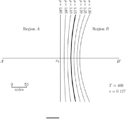
Fig. 6.3
Line boundary
between two regions for
different values of
ρ
1
ρ
s
ln
x
B
ρ
ð
ln
x
A
Þ
¼
ð
6
:
10
Þ
This is a constrained version of Eq. (
6.5
), which is used to specify the boundary
between the two regions.
An example is given in Fig.
6.3
, where
T
400 (the mileage between
A
0
and
B
0
)
¼
and
s
0.127 (the estimated constant for the US). The diagram indicates the
boundaries between regions
A
and
B
for various values of
¼
1 we have
the special case where the density functions of the two regions are identical, and the
boundary between the two is shown as a straight line, perpendicular to the line
A
0
B
0
at
x
h
, the halfway distance between the two metropolitan areas. The bold line
indicates the boundary for the case
ρ
. When
ρ
¼
1.15. This boundary intersects the line
A
0
B
0
where the distances from the two metropolitan areas are
x
*
ρ
¼
¼
236 and
x
*
164.
Two general features of the boundaries in Fig.
6.3
are of interest. First (when
ρ>
¼
1), the boundary is displaced from the halfway point toward the smaller
metropolitan area
B
0
, and the greater the value of
ρ
, the more pronounced is this
displacement. Second (again when
1), the boundary is convex to the larger
metropolitan area
A
0
, and the greater the value of
ρ>
, the greater is the extent of this
convexity. A discussion of additional aspects of the boundary between regions
A
and
B
is contained in Appendix 6.2.
ρ
6.5.2 Two Modifications
In this approach to specifying the boundary, each density function assumes radial
symmetry throughout its region, i.e., for every distance
x
there is no directional
variation in
M
(
x
). In the absence of such symmetry,
M
(
x
) is simply a mean value, so