Geology Reference
In-Depth Information
temperature changes in high latitudes would be
greater than in equatorial regions. Portions of the
globe will experience some benefit from climate warm-
ing (e.g., longer growing and ice-free transportation sea-
sons); others will not. Adjusting to climate change may
be difficult for some sectors (e.g., agriculture, urban
water and sewage systems, and river and lake trans-
portation). Current responses to rising greenhouse
gases (GHG) probably will not prevent C0
2
from
exceeding 700 ppm.
3. Calculate the average annual rate of CO
z
increase (in
ppm/yr) between 1960 and 1980?
4. Using Figure 18.8, estimate the C0
2
concentration in the
year 2020 by linear projection. Extend the C0
2
line by plac-
ing a ruler on the line joining 1980 and the last point (2004).
Draw this line through the year 2020. The C0
2
value
expected at that time by this technique is
ppm.
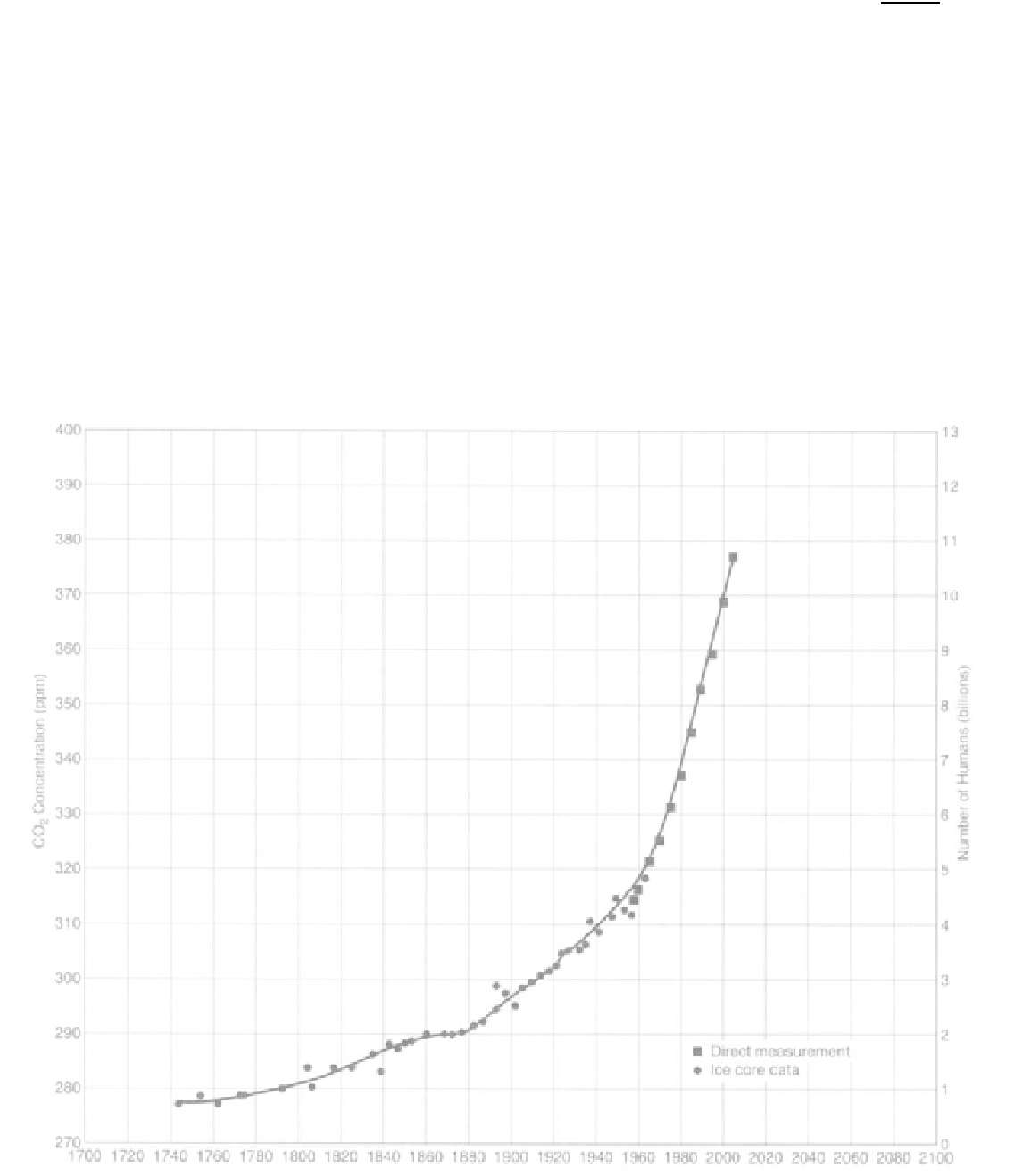
QUESTIONS 18, PART C
Study Figure 18.8 and then answer the following questions.
5.
Using the data in Table 18.1, plot the change in world pop-
ulation between 1700 and 2005 on the same figure as C0
2
increase (Figure 18.8). Use the right axis for the population
scale. Write a revised caption for Figure 18.8 here.
1.
Where were the data collected that are shown in the graph?
2.
According to Figure 18.8, when did C0
2
levels first begin
to increase?
6.
Note the shape of the two curves in Figure 18.8. What is
the apparent cause-effect relationship between the two?
1700 1720 1740 1760 1780 1800 1820 1840 1860 1880 1900 1920 1940 1960 1980 2000 2020 2040 2060 2080 2100
FIGURE 18.8
C0
2
concentration in the atmosphere. Squares are direct atmospheric measurements at Mauna Loa and circles are mea-
surements from ice cores from Siple Station, Antarctica.
(Modified from Siegenthaler and Oeschger, 1987; data also from Keeling, 1976, and Mauna Loa Observatory.)