Biomedical Engineering Reference
In-Depth Information
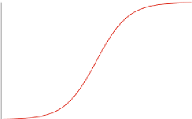
Fig. 4
Graph of the logistic
function, (
8
)
1
0.5
0
−
6
−
4
−
2
0
2
4
6
whose derivative is
e
t
p
lg
.t /
D
D
p
lg
.1
p
lg
/;
(9)
e
t
/
2
.1
C
whose graphic can be seen in Fig.
4
.
For (
8
) to approximate (
2
) some adjustments must be made. Transforming the
range d
W
W
Œd
1
;d
2
to t
Œ
5; 5 of (
8
) leads to
d
d
1
C
10
d
2
d
2
t.d/
D
(10)
d
1
2
and
10
d
2
t
0
.d /
D
d
1
:
(11)
To p
ad
.d
1
/
Q
p
YL
.d
1
/ and p
ad
.d
2
/
0,(
8
)and(
9
) are transformed into
1
p
lg
.t .d //
2
d
1
D
p
ad
.d /
(12)
and
2
d
1
p
0
ad
.d /
t
0
.d / p
lg
.t .d //:
D
(13)
Finally, a value for p
c
0
in (
5
) is chosen, such that p
.0/
DQ
p
c
0
. By stressing (
5
)
and (
12
)inside(
3
)atd
D
0,
2
d
1
DQ
2
d
1
:
p
.0/
D
p
c
0
p
c
0
,
p
c
0
DQ
p
c
0
C
(14)
With p
c
0
of (
14
)in(
5
)and(
12
), (
3
) can be fully rewritten,
(
1
)
:
p
c
0
C
e
ln
100
d
2
d
1
2
d
1
1
p
ad
.d /
D
C
(15)
d
1
d
1
h
d
d
1
C
d
2
2
i
10
d
2
e
1
C
Equations
3
and
4
are illustrated in Figs.
5
and
6
, respectively.