Graphics Programs Reference
In-Depth Information
functionr=residual(u)%Boundaryresidual.
global XSTART XSTOP H
x = XSTART;
[xSol,ySol] = runKut5(@dEqs,x,inCond(u),XSTOP,H);
r = ySol(size(ySol,1),1) - 2;
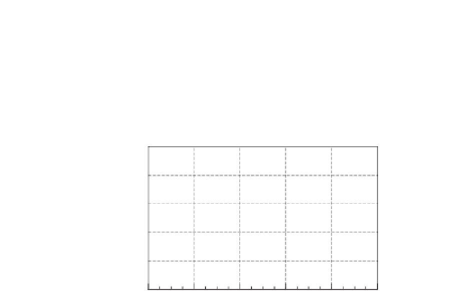
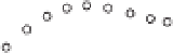
Weskip the rather long printout of the solution and showjust the plot:
8
6
4
2
0
-2
0
1
2
3
4
5
x
Higher-Order Equations
Consider the fourth-orderdifferentialequation
y
(4)
y
,
y
,
y
)
=
f
(
x
,
y
,
(8.4a)
with the boundary conditions
y
(
a
)
y
(
b
)
y
(
a
)
=
α
1
=
α
2
y
(
b
)
=
β
1
=
β
2
(8.4b)
To solve Eq. (8.4a) with the shooting method, we need four initialconditions at
x
a
,
only twoofwhich arespecified. Denoting the two unknown initial values by
u
1
and
u
2
, wehave the set of initialconditions
=
y
(
a
)
y
(
a
)
y
(
a
)
y
(
a
)
=
α
1
=
u
1
=
α
2
=
u
2
(8.5)
If Eq. (8.4a) is solvedwith the shooting methodusing the initialconditions in
Eq. (8.5), the computedboundary values at
x
=
b
depend on the choice of
u
1
and
u
2
.
Weexpress this dependence as
y
(
b
)
y
(
b
)
=
θ
1
(
u
1
,
u
2
)
=
θ
2
(
u
1
,
u
2
)
(8.6)
The correct choice of
u
1
and
u
2
yields the givenboundary conditions at
x
=
b
; that is,
itsatisfies the equations
θ
1
(
u
1
,
u
2
)
=
β
1
θ
2
(
u
1
,
u
2
)
=
β
2


Search WWH ::

Custom Search