Interpolation and Curve Fitting - Numerical Methods in Engineering with MATLAB - page 115

4.00000 3.88327 3.88328

4.50000 3.64994 3.64995

5.00000 3.39411 3.39411

5.50000 3.11735 3.11735

6.00000 2.82137 2.82137

6.50000 2.50799 2.50799

7.00000 2.17915 2.17915

7.50000 1.83687 1.83688

8.00000 1.48329 1.48328

3.3 Interpolation with Cubic Spline

If there are morethan a fewdatapoints, a cubicspline ishard to beat as aglobal
interpolant. It isconsiderably“stiffer” than a polynomial in the sense that ithas less
tendency to oscillate betweendatapoints.

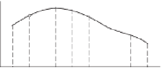
Elastic strip

y

Figure 3.6. Mechanical model of naturalcubicspline.

Pins (data points)
x

Themechanicalmodel of a cubicspline is shown inFig. 3.6. It is a thin,elasticstrip
that is attachedwith pinstothedatapoints.Because the strip is unloadedbetween the
pins, each segment of the splinecurve is a cubic polynomial—recall frombeam the-
ory that the differentialequation for the displacementofabeam is d 4 y dx 4 ( E I ),

so that y ( x ) is a cubicsince the load q vanishes.At the pins, the slope and bending
moment(and hence the second derivative) arecontinuous. There is no bending mo-
ment at the twoend pins; hence the second derivative of the spline iszero at the end
points.Since these end conditions occur naturallyinthe beam model, the resulting
curve isknown as the natural cubic spline . The pins, i.e., the datapoints, arecalled
the knots of the spline.

/ = q /

y

f ( )

i, i + 1

Figure 3.7. Cubicspline.

y

y

y

y y

i

- 1

i

i

+ 1

1 2

y

n

- 1

y

n

x

x xx x x

x x 1

i i

+ 1 + 1 + 1

2

i

- 1

n - 1 n

Figure 3.7 shows a cubicsplinethatspans n knots.We use the notation f i , i + 1 ( x )
for the cubic polynomialthatspans the segment between knots i and i + 1. Note