Data Reduction - Data Preprocessing in Data Mining - page 148

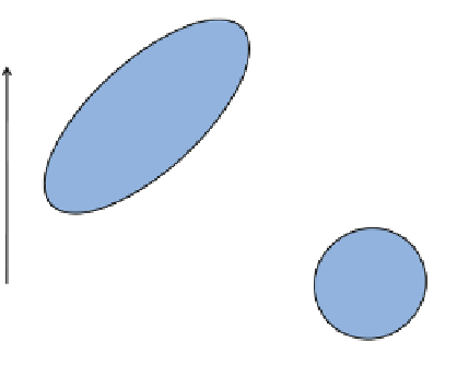
Fig. 6.2 Factors are independent unit normals that are scaled, rotated and translated to compose
the inputs

To find F and L , three common restrictions on their statistical properties are
adopted: (1) all the factors are independent, with zero mean and variance of unity,
(2) all the error terms are also independent, with zero mean and constant variance,
(3) the errors are independent of the factors.
There are two methods for solving the factor model equations for the matrix K
and the factors F : (1) the maximum likelihood method and (2) the principal com-
ponent method. The first assumes that original data is normally distributed and is
computationally expensive. The latter is very fast, easy to interpret and guarantees
to find a solution for all data sets.

1. Unlike PCA, factor analysis assumes and underlying structure that relates the
factors to the observed data.
2. PCA tries to rotate the axis of the original variables, using a set of linear trans-
formations. Factor analysis, instead, creates a new set of variables to explain the
covariances and correlations between the observed variables.
3. In factor analysis, a two-factor model is completely different from a three-factor
model, whereas in PCA, when we decide to use a third component, the two first
principal components remain the same.
4. PC is fast and straightforward. However, in factor analyses, there are various
alternatives to performing the calculations and some of them are complicated and
time consuming.

Figure 6.2 exemplifies the process of factor analysis. The differences between
PCA and factor analysis can be enumerated.

6.2.3 Multidimensional Scaling

Let us assume N points, and that we know the distances between the pairs of points,
d ij , for all i , j = 1 ,..., N . Moreover, we do not know the precise coordinates of the