Information Technology Reference
In-Depth Information
This results in 15,300 runs. The iteration limit was set at 1000 iterations for
each run.
Figure 2 plots the results for the different values of
α
and
β
. The vertical axis
indicate the average relative deviation from the best known feasible solution for
each instance. One of the first observations we can make from the plot is that the
parameter
α
has more influence over the solution quality than
β
does. This of
course is a normal behavior in many GRASP implementations; however, we can
also observe that the best possible value of this
α
depends on the instance size.
For the smaller instances, the best solutions were obtained when
α
lies around
0.7. As the size of the instances grows, we can see how this best value of
α
goes down to around 0.20 for the medium-size instances, and 0.03 for the large-
size instances. This means that reducing diversity in favor of more greedy-like
solutions as instances get large provides a better strategy for finding solutions
of better quality. For the remainder of the experiments we fixed
α
at 0.70, 0.20,
and 0.03 for the small-, medium-, and large-size instances, respectively.
In the following experiment, we try to determine the effect that the step
size
Δβ
has on algorithmic performance. While it is true that providing a finer
discretization (i.e., reducing the step size
Δβ
) could lead to more and better
solutions, it is also true that the computational burden increases. Moreover,
when the step size is suciently small, solutions obtained from different values
of
β
will look alike, resulting in very little gain. Therefore, the purpose of this
experiment is to investigate this effect. To this end, we run the heuristic fixing
Δβ
at different values as
Δβ
=1
/x
with
x
∈{
1
,
2
,...,
10
}
. The iteration limit
was set at 1000.
12.0%
10.0%
8.0%
6.0%
Small
Medium
Large
4.0%
2.0%
0.0%
1/10 1/9
1/8
1/7
1/6
1/5
1/4
1/3
1/2
1
'
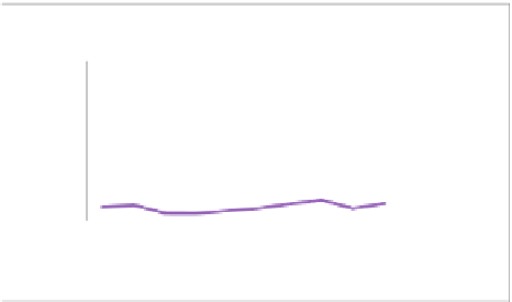
Fig. 3.
Algorithm behavior as a function of
Δβ
Figure 3 displays the results plotting in the vertical axis the average deviation
from the best known solution for every instance. The horizontal axis shows the
different values of
Δβ
. As can be seen from Figure 3, for the large-size instances
the choice of
Δβ
did not have much impact; however, a slight improvement is
observed at values around 1/8, which in fact matches the best value found for
the small- and medium-size instances.