Generation of Computational Mesh for Haemodynamics Analysis - Computational Hemodynamics: Theory, Modelling and Applications - page 156

Mesh
spacing

Δ x i

Δ y j

Grid point

Uniform rectangular mesh in 2D (with its coordinate grid points), and in 3D

a

Coarser mesh away
from the vertical wall
boundaries

Finer mesh concentrated near
the vertical wall boundaries

Δ x 3 Δ x 2 Δ x 1

Δ x 5 Δ x 4

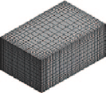
Non-uniform rectangular mesh in 2D
(with its coordinate grid points near the wall) and 3D

b

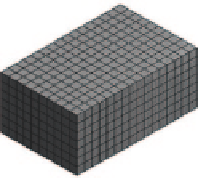
Fig. 6.2 a A uniform and b non-uniform structured mesh in 2D and 3D for a simple rectangular
geometry. Note the evenly distributed grid points in the uniform mesh in contrast to the biased
concentration of cells near the wall for a non-uniform structured mesh

As an alternative a similar type of structured mesh called a body-fitted mesh can
be applied. This approach centres on mapping the distorted region in physical space
onto a rectangular curvilinear coordinate space through a transform coordinate
function. Applying a body-fitted mesh to the 90 o bend geometry, the walls coincide
with lines of constant η (see Fig. 6.4 ). The path length from the vertices A to B , and
D to C , then correspond to specific values of ξ in the computational domain. In this
example we see that η is constant but there is a stretching of ξ in the curved region.
A transformation must be defined such that there is a one-to-one correspondence
between the rectangular mesh in the computational domain and the curvilinear
mesh in the physical domain. The algebraic forms of the governing equations for
fluid flow are carried out in the computational domain which has uniform spacing
of ∆ ξ and uniform spacing of ∆η . Computed information is then directly fed back