Computational Fluid Structure Interaction - Computational Hemodynamics: Theory, Modelling and Applications - page 137

elements A 31 , A 41 , …., A n 1 in the first column of matrix A are treated similarly by
repeating this process down the first column (e.g. Row3- Row1 × A 31 / A 11 ), so that
all the elements below A 11 are reduced to zero. The same procedure is then applied
for the second column, (for all elements below A 22 ) and so forth until the process
reaches the n -1 th column. Note that at each stage we need to divide by A nn and there-
fore it is imperative that the value is non-zero. If it is not, then row exchange with
another row below that has a non-zero needs to be performed.
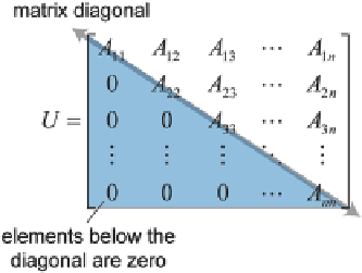
After this process is complete, the original matrix A becomes an upper triangu-
lar matrix that is given by:

AAA A
AA A
A

11 12 13 1 n

0

22 23 2 n

U = 0 A

33 3 n

000 A

nn

All the elements in the matrix U except the first row differ from those in the original
matrix A and our systems of equations can be rewritten in the form:

UB φ=

The upper triangular system of equations can now be solved by the Back Substitu-
tion process. The last row of the matrix U contains only one non-zero coefficient,
A nn , and its corresponding variable ϕ n is solved by

B
U

n

φ =

n

nn

The second last row in matrix U contains only the coefficients A n- 1, n and A nn and,
once ϕ n is known, the variable ϕ n− 1 can be solved. By proceeding up the rows of the
matrix we continue substituting the known variables and ϕ i is solved in turn. The
general form of equation for ϕ i is expressed as:

n

∑

B − A φ

i ij j

ji =+ 1

φ = (5.76)

i

A

ii

It is not difficult to see that the bulk of the computational effort is in the forward
elimination process; the back substitution process requires less arithmetic opera-
tions and is much less costly. Gaussian elimination can be expensive especially for