Computational Fluid Structure Interaction - Computational Hemodynamics: Theory, Modelling and Applications - page 131

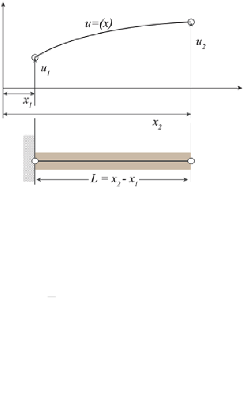
Fig. 5.36 A single 1D finite
bar element with forces
applied at the ends of the bar

(5.60)

ux NxuNxu () () = + () [ {} = N u

1 1 2 2

where [ ] is a row matrix and {} is a column matrix.
The shape functions for each node are

x x − xx −

x x

2 1

N = = − 1 N = = (5.61)

1 2

xx − L xx L −

2 1 2 1

which provides a linear interpolation from node-1 to node-2, since it produces
N 1

= for x = x 1 , and N 1 = for x = x 2 , and similarly for node-2.
The continuous displacement function represented by the discretisation becomes

x
L

x
L

+ ux () [ {} = N u = 1 − u u

(5.62)

1 2

where [ ] is a row matrix of the interpolation functions, and {} is a column matrix
of the nodal displacements. We now determine the relation between the nodal dis-
placements and applied forces to obtain the stiffness matrix for the bar element. The
fundamental equation for deflection δ of an elastic bar having modulus of elastic-
ity E , length L and uniform cross-sectional area A when subjected to axial load P is
given by δ= PL / AE and the equivalent spring constant is

P AE

(5.63)

k

==

L

To compute the nodal displacements from some given loading condition on the ele-
ment we obtain the necessary equilibrium equations relating the displacements to
applied forces. Firstly the strain-displacement relation is